Vehicle Detection (Code)

The goal of this project is to identify vehicles in a video from a front-facing camera on a car. At first the pipeline is developed on a series of individual images, and later the result is applied to a video stream.

The tools used are (in the following order):

• Perform a Histogram of Oriented Gradients (HOG) feature extraction on a labeled training set of images and train a Linear SVM Classifier
• Apply a Color Transform and append Binned Color Features, as well as histograms of color, to the HOG feature vector.
• Implement a Sliding-Window technique and use the trained classifier to search for vehicles in images.
• Create a Heat Map of recurring detections frame by frame to reject outliers and follow detected vehicles.
• Estimate a Bounding Box for vehicles detected.

The project is developed using Python and OpenCv. You can download the full code from GitHub.

---

Histogram of Oriented Gradients (HOG)

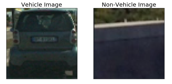
I started by reading in all the vehicle and non-vehicle images. Here is an example of one of each of the vehicle and non-vehicle classes:

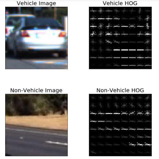
I then explored different color spaces and different skimage.hog() parameters (orientations, pixels_per_cell, and cells_per_block), I grabbed random images from each of the two classes and displayed them to get a feel for what the skimage.hog() output looks like.

The figure below shows an example of a car image and its associated histogram of oriented gradients, as well as the same for a non-car image using the RGB color space and HOG parameters of orientations=8, pixels_per_cell=(8, 8) and cells_per_block=(2, 2):

I used the following helper functions to extract the HOG features:

def get_hog_features(img, orient, pix_per_cell, cell_per_block,
                        vis=False, feature_vec=True):
    # Call with two outputs if vis==True
    if vis == True:
        features, hog_image = hog(img, orientations=orient,
                                  pixels_per_cell=(pix_per_cell, pix_per_cell),
                                  cells_per_block=(cell_per_block, cell_per_block),
                                  block_norm= 'L2-Hys',
                                  transform_sqrt=False,
                                  visualize=vis, feature_vector=feature_vec)
        return features, hog_image
    # Otherwise call with one output
    else:      
        features = hog(img, orientations=orient,
                       pixels_per_cell=(pix_per_cell, pix_per_cell),
                       cells_per_block=(cell_per_block, cell_per_block),
                       block_norm= 'L2-Hys',
                       transform_sqrt=False,
                       visualize=vis, feature_vector=feature_vec)
        return features

and the Color Transform:

def convert_color(image, color_space):
    if color_space != 'RGB':
        if color_space == 'HSV':
            feature_image = cv2.cvtColor(image, cv2.COLOR_RGB2HSV)
        elif color_space == 'LUV':
            feature_image = cv2.cvtColor(image, cv2.COLOR_RGB2LUV)
        elif color_space == 'HLS':
            feature_image = cv2.cvtColor(image, cv2.COLOR_RGB2HLS)
        elif color_space == 'YUV':
            feature_image = cv2.cvtColor(image, cv2.COLOR_RGB2YUV)
        elif color_space == 'YCrCb':
            feature_image = cv2.cvtColor(image, cv2.COLOR_RGB2YCrCb)
    else:
        feature_image = np.copy(image)
    return feature_image

def bin_spatial(img, size=(32, 32)):
    color1 = cv2.resize(img[:,:,0], size).ravel()
    color2 = cv2.resize(img[:,:,1], size).ravel()
    color3 = cv2.resize(img[:,:,2], size).ravel()
    return np.hstack((color1, color2, color3))

def color_hist(img, nbins=32):    #bins_range=(0, 256)
    # Compute the histogram of the color channels separately
    channel1_hist = np.histogram(img[:,:,0], bins=nbins)
    channel2_hist = np.histogram(img[:,:,1], bins=nbins)
    channel3_hist = np.histogram(img[:,:,2], bins=nbins)
    # Concatenate the histograms into a single feature vector
    hist_features = np.concatenate((channel1_hist[0], channel2_hist[0], channel3_hist[0]))
    # Return the individual histograms, bin_centers and feature vector

    return hist_features

---

Classifier Training

I trained a linear SVM using the default classifier parameters and using HOG Features, Spatial Intensity and Color Intensity Histogram Features.

I settled on my final choice of parameters based upon the performance of the SVM classifier.

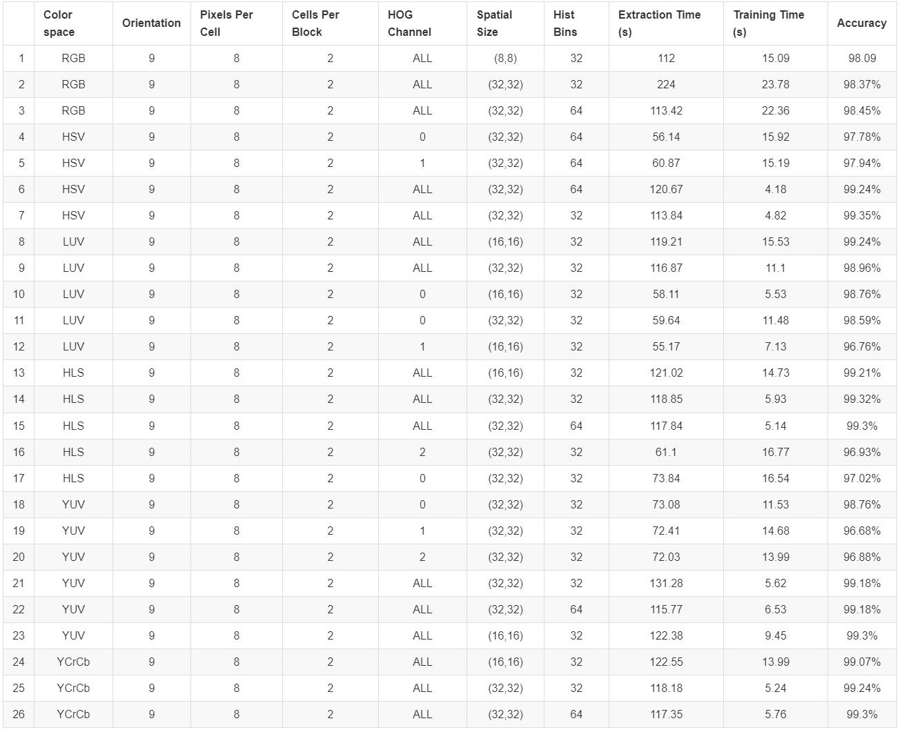
Specifically, the final parameters chosen were: HSV color space, 9 orientations, 8 pixels per cell, 2 cells per block, ALL channels of the HOG space, (32, 32) spatial size and 32 histogram bins. The classifier performance of each of the configurations are summarized in the table below:

Both configurations number 7 and number 26 give good results on the final video. I chose the number 7 because despite being more wiggly, it’s capable of identifying cars on the other side of the road.

Sliding Window Search

The method combines HOG feature extraction with a sliding window search, but rather than performing feature extraction on each window individually, the HOG features are extracted just once for the entire region of interest (i.e. lower half of each frame of video) and subsample that array for each sliding window.

I decided to search the lower half of each frame of video at different scales. The following images show the configurations of all search windows in the final implementation, for small scale = 1.0, 1.5, 2.0 and 3.0:

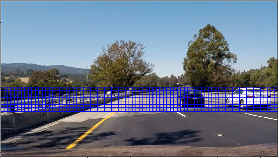
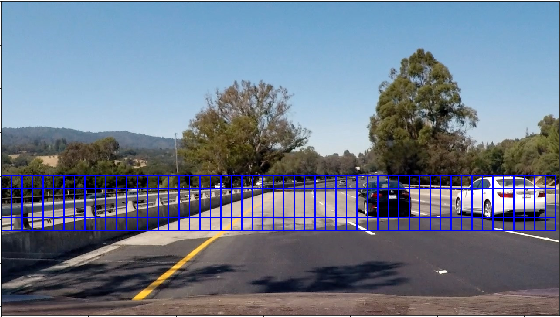
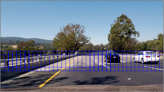
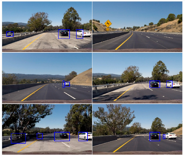
Ultimately I searched on four scales using HSV 3-channel HOG features plus spatially binned color and histograms of color in the feature vector, which provided a nice result. Here is the result on some test images:

---

Video Implementation

I recorded the positions of positive detections in each frame of the video. From the positive detections I created a heatmap and then thresholded that map to identify vehicle positions. I then used scipy.ndimage.measurements.label() to identify individual blobs in the heatmap. I then assumed each blob corresponded to a vehicle. I constructed bounding boxes to cover the area of each blob detected.

Here is a frames and its corresponding heatmap:

Results

Here’s the result of the pipeline applied to all the test images included in the project:

Shortcomings with current pipeline

The pipeline fails with cars that surpass each other occluding the view, they are hard to tell apart and detected as a single entities. When the cars are very far the detector needs to run at small scale in order to find them, but this creates a lot of small positive detections.

Possible improvements

• Including more data: although the test accuracy of the classifier is high, it is very likely this is overfitted because the training dataset contains some time series data.
• Determine vehicle location and speed to predict its location in subsequent frames.
• Trying out convolutional neural network to implement the image classifier and see whether it gives better results.