Traffic Sign Classifier (Code)

The goals of this project is to design and implement a deep learning model that learns to recognize traffic signs. The dataset used is the German Traffic Sign Dataset .
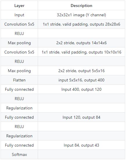
The starting point is the LeNet-5 implementation, the only changes are the number of classes and the preprocessing.

The steps followed are:

• Load the data set (see above for links to the project data set)
• Explore, summarize and visualize the data set
• Design, train and test a model architecture
• Use the model to make predictions on new images
• Analyze the softmax probabilities of the new images

The project is developed using Python and OpenCv. You can download the full code from GitHub.

---

Load data set

I used a pickled dataset in which the images have already been resized to 32x32. It contains a training, validation and test set.

training_file = './train.p'
validation_file= './valid.p'
testing_file = './test.p'

with open(training_file, mode='rb') as f:
    train = pickle.load(f)
with open(validation_file, mode='rb') as f:
    valid = pickle.load(f)
with open(testing_file, mode='rb') as f:
    test = pickle.load(f)

X_train, y_train = train['features'], train['labels']
X_valid, y_valid = valid['features'], valid['labels']
X_test, y_test = test['features'], test['labels']

The pickled data is a dictionary with 4 key/value pairs:

• features is a 4D array containing raw pixel data of the traffic sign images, (num examples, width, height, channels).
• labels is a 1D array containing the label/class id of the traffic sign.
• sizes is a list containing tuples, (width, height) representing the original width and height the image.
• coords is a list containing tuples, (x1, y1, x2, y2) representing coordinates of a bounding box around the sign in the image.

Data Set Summary & Exploration

I used the numpy library to calculate summary statistics of the traffic signs data set:

• The size of training set is 34799 samples
• The size of the validation set is 4410 samples
• The size of test set is 12630 samples
• The shape of a traffic sign image is (32, 32, 3)
• The number of unique classes/labels in the data set is 43

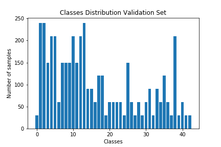
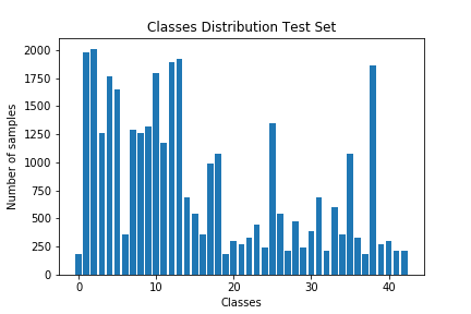
Here is an exploratory visualization of the data set. They are bar charts showing the data distribution for training, validation and test set is the same.

---

Design and Test a Model Architecture

Data Pre-processing

As a first step, I decided to convert the images to YUV space and keep only the Y channel as suggested in this published model because the color feature is not relevant in this task and it would only increase the computational cost.

After that, I applied a Histogram Equalizer to normalize the brightness and increase the contrast of the image.

X_train_proc = np.zeros((X_train.shape[0], X_train.shape[1], X_train.shape[2], 1))
for i in range(X_train.shape[0]):
    img_yuv = cv.cvtColor(X_train[i], cv.COLOR_BGR2YUV)
    y,_,_ = cv.split(img_yuv)
    clahe = cv.createCLAHE(clipLimit=2.0, tileGridSize=(8,8))
    X_train_proc[i,:,:,0] = clahe.apply(y)

Here is an example of a traffic sign image before and after pre-processing.

I decided to do data augmentation to increase the diversity of data available for training models, without actually collecting new data. Samples were randomly perturbed in position ([-2,2] pixels) and rotation ([-15,+15] degrees), as described in the published model.

Here is an example of an original image and an augmented image:

The difference between the original data set and the augmented data set is an increment in the number of images, which now have only one channel.

Following, I normalized the image data because it makes convergence faster while training the network.

X_train_proc = (aug_X_train - np.mean(aug_X_train))/np.std(aug_X_train)
X_valid_proc = (X_valid_proc - np.mean(X_valid_proc))/np.std(X_valid_proc)
X_test_proc = (X_test_proc - np.mean(X_test_proc))/np.std(X_test_proc)

As a last step, I shuffled the training set otherwise the ordering of the data might have an effect on how well the network trains.

Final Model Architecture

Training hyperparameters

I trained the model using an Adam Optimizer, a learning rate of 0.001 ( it tells tensorflow how quickly to update the network’s weights and this is a good default value), a dropout rate of 0.1 and batch size of 128.

The batch size variable tells tensorflow how many training images to run through the network at a time. The larger the batch size, the faster our model will train but our processor may have a memory limit on how large a batch it can run.

My final model results were:

• validation set accuracy of 0.943
• test set accuracy of 0.925

An iterative approach was chosen:

• The starting point was the LeNet Neural Network because it performs well on recognition tasks. I adapted it to my model with 43 final outputs.
• Initially, I noticed that this architecture overfitted the original training set and I introduced Dropout Regularization after the first two Dense layers.
• After a few trial and error I was able to tune both the dropout rate and the learning rate to 10% and 0.001.

---

Test a Model on New Images

I chose five German traffic signs on the web to test my model on:

All these images maybe challenging to classify because:

• they include much more background then the training images
• the background is very different from the one in the training images
• one image contains copyright trademarks

Here are the results of the prediction:

Top 5 labels for Speed limit (30km/h):

• Speed limit (30km/h) with prob = 0.91
• Speed limit (50km/h) with prob = 0.09
• End of speed limit (80km/h) with prob = 0.00
• Speed limit (80km/h) with prob = 0.00
• Speed limit (20km/h) with prob = 0.00

Top 5 labels for Bicycles crossing:

• Bicycles crossing with prob = 0.99
• Children crossing with prob = 0.01
• Slippery road with prob = 0.00
• Bumpy road with prob = 0.00
• Speed limit (60km/h) with prob = 0.00

Top 5 labels for Beware of ice/snow:

• Slippery road with prob = 0.95
• Beware of ice/snow with prob = 0.04
• Wild animals crossing with prob = 0.01
• Double curve with prob = 0.00
• Road work with prob = 0.00

Top 5 labels for Ahead only:

• Ahead only with prob = 1.00
• Turn left ahead with prob = 0.00
• No vehicles with prob = 0.00
• Speed limit (60km/h) with prob = 0.00
• Turn right ahead with prob = 0.00

Top 5 labels for No passing:

• No entry with prob = 1.00
• Stop with prob = 0.00
• End of all speed and passing limits with prob = 0.00
• End of no passing with prob = 0.00
• No passing with prob = 0.00

The model was able to correctly guess 3 of the 5 traffic signs, which gives an accuracy of 60%.

Here’s the snippet of the code for making predictions:

probability_prediction = tf.nn.softmax(logits=logits)

def predict(X_data):
    num_examples = len(X_data)
    sess = tf.get_default_session()
    predictions = list()
    for offset in range(0, num_examples, BATCH_SIZE):
        batch_x = X_data[offset:offset+BATCH_SIZE]
        predictions.extend( sess.run(probability_prediction, feed_dict={x: batch_x}))

    return predictions

---

Shortcomings with the current pipeline

A shortcoming could be the way fake data have been generated, using Keras of Tensorflow might end up with better data augmentation

---

Possible improvements

• Use a different network architecture or change the dimensions of the Le-Net layers
• Graph validation and training error to better tune the hyperparameters and make sure the network doesn’t overfit the data.
• Run the network for a higher number of epochs (if you have a big enough GPU)