Sensor Fusion and Tracking
The purpose of this post is to explain my Implementation of the open-source project for the course in the Udacity Self-Driving Car Engineer Nanodegree Program : Sensor Fusion and Tracking and build up some intuition about the process. There won’t be any snippets from the source code since we only want to build a high level understanding of why we do what we do.
Abstract
This work proposes a method to detect and track vehicles from LiDAR maps guided by RGB images. A multitude of applications depend on the awareness of their surroundings to reason and react accordingly, and the use of LiDAR is crucial for both autonomous vehicles and robotics. This fusion method takes advantage of RGB guidance from a monocular camera to leverage object information and accurately track vehicle from point clouds. This improves the accuracy significantly.
A deep-learning approach is used to detect vehicles in LiDAR data based on a birds-eye view perspective of the 3D point-cloud, followed by an extended Kalman filter used to track vehicles over time, based on the lidar detections fused with camera detections. Two models (Resnet and Darknet) are implemented and their performance evaluated based on precision and recall.
This project is based on the project for the course in the Udacity Self-Driving Car Engineer Nanodegree Program: Sensor Fusion and Tracking. You can download the full code from GitHub.
Introduction
Multiple Object Tracking (MOT) is a robot vision problem with the goal of analyzing videos in order to detect and track objects belonging to one or more categories, without any prior knowledge about the appearance and number of targets [3]. 3D perception as well as precise 3D object detection and tracking are important components in state-of-the-art driving systems [2].
This work will focus on self-driving cars, while using LiDAR and monocular RGB images. Here, it is desirable to accurately detect and differentiate objects close as well as far away, and the LiDAR provides the necessary information in the form of a point cloud of its surroundings.
The reason 3D detection on point-clouds is challenging is threefold: first, point-clouds are sparse, and most regions of 3D space are without measurements [5]. Second, the resulting output is a three-dimensional box that is often not well aligned with any global coordinate frame. Third, 3D objects come in a wide range of sizes, shapes, and aspect ratios.
In this project, measurements from LiDAR and camera are fused to track vehicles over time using the Waymo Open Dataset [9].
The contributions of this paper are:
- Object detection: a deep-learning approach is used to detect vehicles in LiDAR data based on a birds-eye view perspective of the 3D point-cloud. Also, a series of performance measures is used to evaluate the performance of the detection approach.
- Object tracking: an extended Kalman filter is used to track vehicles over time, based on the lidar detections fused with camera detections. Data association and track managementare implemented as well.
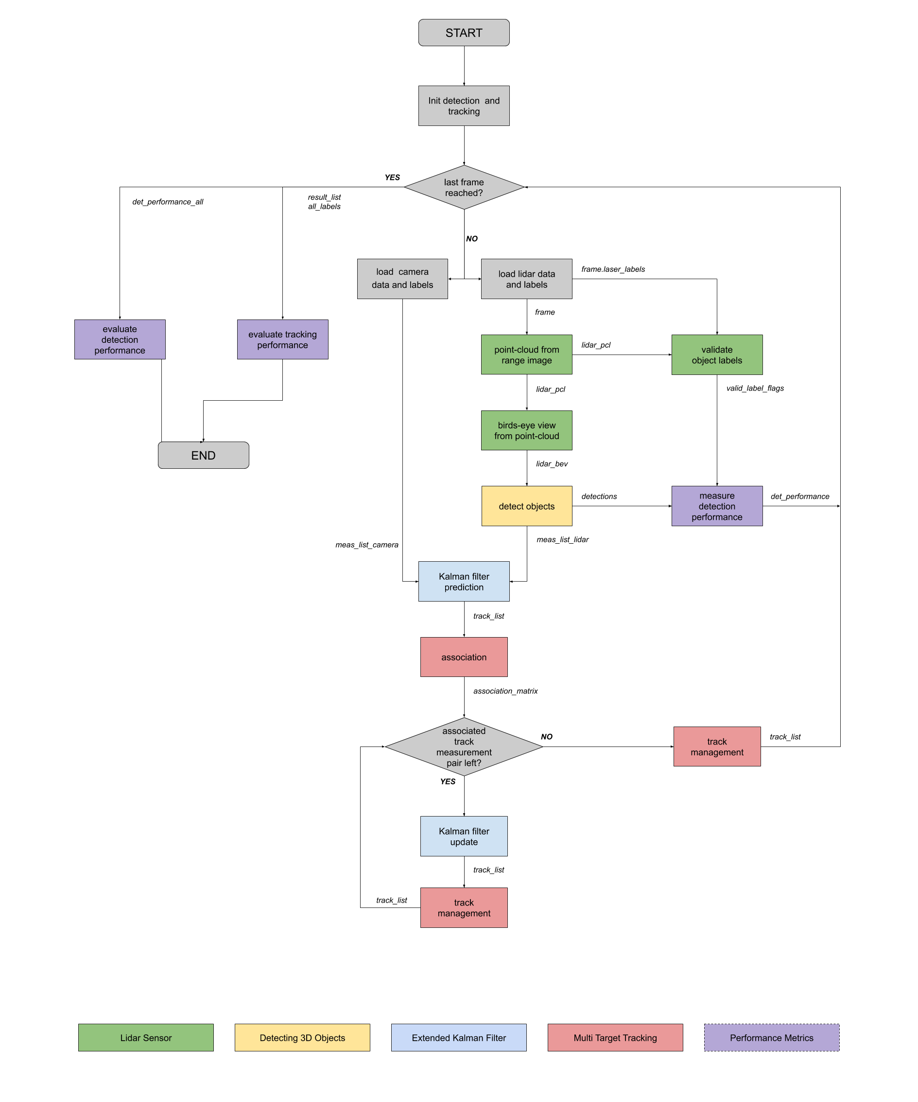
The diagram in the following figure contains an outline of the data flow and of the individual steps that make up the algorithm. Two different models based on a Resnet and Darknet architecture are adopted and their performance on both object detection and tracking evaluated using precision and recall as metrics.
Method
The method proposed acts on a projection of a 3D point cloud to a 2D plane, namely birds eye view.
Object Detection
A deep-learning approach is used to detect vehicles in LiDAR data based on a birds-eye view perspective of the 3D point-cloud.
From Range Image to Point Cloud. Since in the Waymo Open Dataset the point cloud of each LiDAR is encoded as a range image [9], converting from a range image to a point cloud is the first step of the pipeline.
A range image represents a LiDAR point cloud in the spherical coordinate system based on the following rules:
- Each row corresponds to an inclination. Row 0 (top of the image) corresponds to the maximum inclination.
- Each column corresponds to an azimuth. Column 0 (left of the image) corresponds to -x-axis (i.e. the opposite of forward direction). The center of the image corresponds to the +x-axis (i.e. the forward direction). Note that an azimuth correction is needed to make sure the center of the image corresponds to the +x-axis.
To compute the conversion we first estimate the inclination angle for each beam in the range image; we then convert the range image to polar coordinate using the camera projection extrinsic parameters provided.
The LiDAR spherical coordinate system is based on the Cartesian coordinate system in LiDAR sensor frame. A point (x, y, z) in LiDAR Cartesian coordinates can be uniquely translated to a (range, azimuth, inclination) tuple in LiDAR spherical coordinates.Hence, ultimately we convert polar coordinates to Cartesian coordinates before stacking the point cloud and LiDAR intensity vertically.
A preview of the range image

as well as its point cloud representation
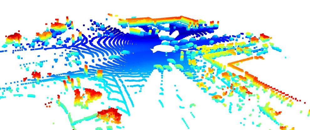
are visible here.
Birds-eye View of LiDAR Data. After obtaining the point cloud, we create its Birds-Eye View perspective (BEV). The crucial part is converting the LiDAR points from sensor coordinates to BEV-map coordinates, which can be computed since each sensor comes with an extrinsic transformation that defines the transform from the sensor frame to the vehicle frame.
A comparison between the two coordinate systems is shown in the following image: the LiDAR (or vehicle) coordinate system is displayed in yellow, while the image coordinate system in blue. In the vehicle system the x-axis is positive forward, the y-axis is positive to the left, and the z-axis is positive upward. For the image coordinate system instead the x-axis is positive to the right and the y-axis is positive downward. Not only the axes of the two systems are inverted, but their directions are opposite, as well as their origin shifted (the LiDAR point cloud is centered at the position of the vehicle while the image has its origin at the top left corner).
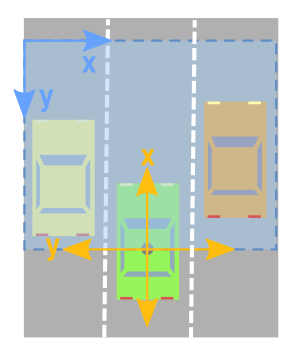
To capture fine details and recognize objects more accurately, instead of casting the values from the point cloud to integers, we modify the level of resolution before assigning them to each pixel.
Finally, to compute the BEV map displayed below, we encode as RGB channels the intensity, height and density layers after normalizing them with the difference between the 1- and 99-percentile to mitigate the influence of outliers.
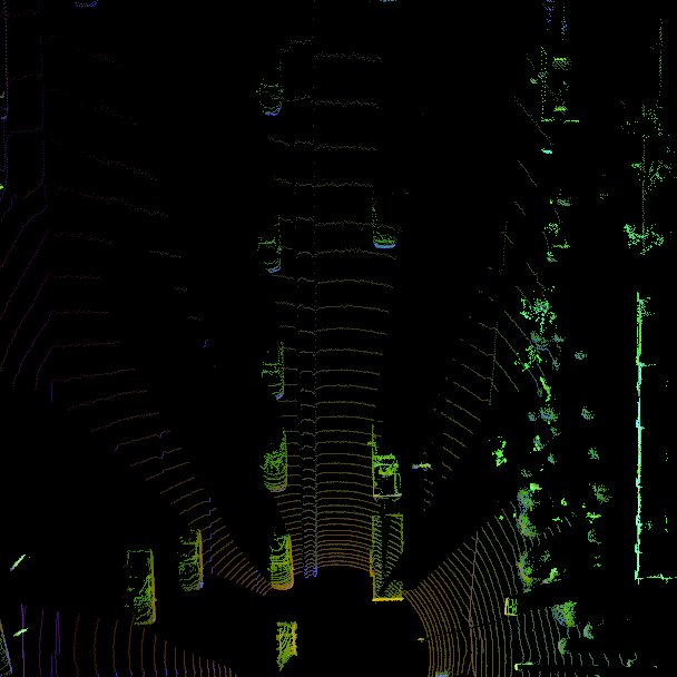
3D Object Detection. The Object Detection framework loads two type of configurations: one from Super Fast and Accurate 3D Object Detection based on 3D LiDAR Point Clouds and the other from Complex-YOLO: Real-time 3D Object Detection on Point Clouds [1, 8]. In the first, the network architecture is based on the ResNet based Keypoint Feature Pyramid Network (KFPN) [4], which provides real-time 3D object detection based on a monocular RGB image [7].
The models take a BEV map encoded by height, intensity, and density of 3D LiDAR point clouds as input, and output the detected bounding boxes in the BEV coordinate space. Before the detections can move along in the processing pipeline, they are converted into metric coordinates in vehicle space.
Performance Evaluation. At the end, we compute various performance measures to assess the object detection: we evaluate the Intersection-Over-Union (IOU) between the ground truth labels and the performed detection to assign a certain detected object to a label based on a threshold. We use this information to compute precision and recall over all frames.
Object Tracking
An Extended Kalman Filter (EKF) is used to track vehicles over time, based on the lidar detections fused with camera detections. The tracking process comprises different modules that linked together perform the task accurately.
Extended Kalman Filter. Kalman filters estimate posterior distributions of robot poses conditioned on sensor data. Exploiting a range of restrictive assumptions (i.e. Gaussian-distributed noise and Gaussian distributed initial uncertainty) they represent posteriors by Gaussians. They offer an elegant and efficient algorithm for localization [10].
The EKF handles nonlinearity by linearizing the system at the point of the current estimate, and then the linear Kalman filter is used to filter this linearized system [6]. The general equations are summarized in the following table.
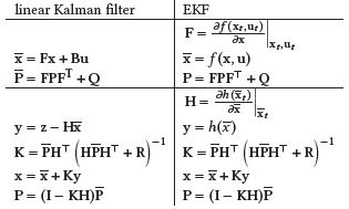
The version implemented here has 6 dimensions (3 for the position (x, y, z) and 3 for the velocity (vx , vy, vz )), and the constant velocity motion model is used for the transition matrix.
Track Management. This module handles the generation of new tracks, removal of old tracks, and it updates the states of the current tracks, based on the information received by the measurements. The track object contains the current state x as well as the state transition matrix P, and they are both initialized based on unassigned measurements previously transformed from sensor to vehicle coordinates. Each track is assigned a score that increases or decreases if it’s associated with a certain measurement or not. Furthermore, a comparison to a certain threshold determines the removal or status update (i.e. from ‘tentative’ to ‘confirmed’) of a specific track.
Association. The track/measurement association is performed using Single Nearest Neighbor Association: an association matrix in computed based on the Mahalanobis distance between each pair. Furthermore, a gate is implemented using the chi square test. The measurement with the smallest entry in the matrix is associated to a particular track.
Measurement. This module initialize the measurement according to the different sensors with the appropriate sensor-to-vehicle projection, making use of homogenous coordinates.
Experiments
Dataset
In this project, measurements from LiDAR and camera are fused to track vehicles over time using the Waymo Open Dataset [9].
Lidar Data. The dataset contains data from five LiDARs - one mid-range LiDAR (top) and four short-range LiDARs (front, side left, side right, and rear).
The following limitations were applied:
- Range of the mid-range LiDARs truncated to a maximum of 75 meters
- Range of the short-range LiDARs truncated to a maximum of 20 meters
- The strongest two intensity returns are provided for all five LiDARs
The point cloud of each LiDAR is encoded as a range image. Two range images are provided for each LiDAR, one for each of the two strongest returns.
3D LiDAR Labels. 3D 7-DOF bounding box labels in the vehicle frame with globally unique tracking IDs are provided. The following objects have 3D labels: vehicles, pedestrians, cyclists, signs.
Camera Data. The dataset contains images from five cameras associated with five different directions. They are front, front left, front right, side left, and side right.
One camera image is provided for each pair in JPEG format. In addition to the image bytes, the vehicle pose, the velocity corresponding to the exposure time of the image center and rolling shutter timing information is provided. This information is useful to customize the LiDAR to camera projection, if needed.
2D Camera Labels. The 2D camera labels are composed of 2D bounding box labels in the camera images. The labels are tightfitting, axis-aligned 2D bounding boxes with globally unique tracking IDs. The bounding boxes cover only the visible parts of the objects. Vehicles, pedestrians, cyclists are the labelled objects.
This project makes use of three different sequences from the Waymo Open Dataset [9], named later as track 1, track 2 and track 3.
The object detection methods used in this project use pre-trained models which have been provided by the original authors as well as pre-computed lidar detections.
Implementation Details
The object detection methods used in this project use pre-trained models which have been provided by the original authors. The code was written in Python 3.7 on a Windows machine. No GPU was used, even though a flag is present to switch hardware.
Results
A series of performance measures is used to evaluate the model at different steps.
Object Detection. Precision and recall are used for the detection approach as suggested in the outline of the project.
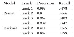
The Resnet detector has a higher precision but a lower recall compared to the model with Darknet over all three tracks. High precision values indicate a low false positive rate, but a low value of recall means that of all the vehicles encountered, only a small percentage was actually identified with respect to the ground truth.
A reason resides in the inaccuracy of the precomputed detection values, which contain many false negatives.
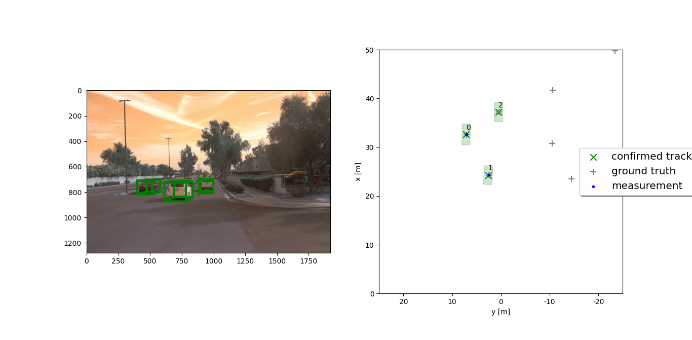
In the image above we can see several ground truths without measurements. Moreover, the detected vehicle 2 despite presenting no measurement is still tracked by the algorithm.
A visual comparison of the detection obtained with the two models is provided in the two images below.
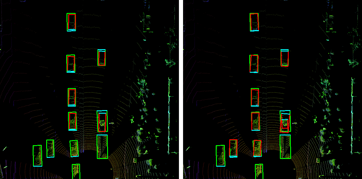
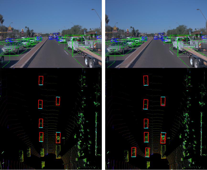
We can see that the model based on Darknet misidentifies a vehicle on the right, but it correctly identifies two vehicles more than the Resnet model in the same frame.
Object Tracking. Finally, the RMSE is used to estimate the tracking performance.
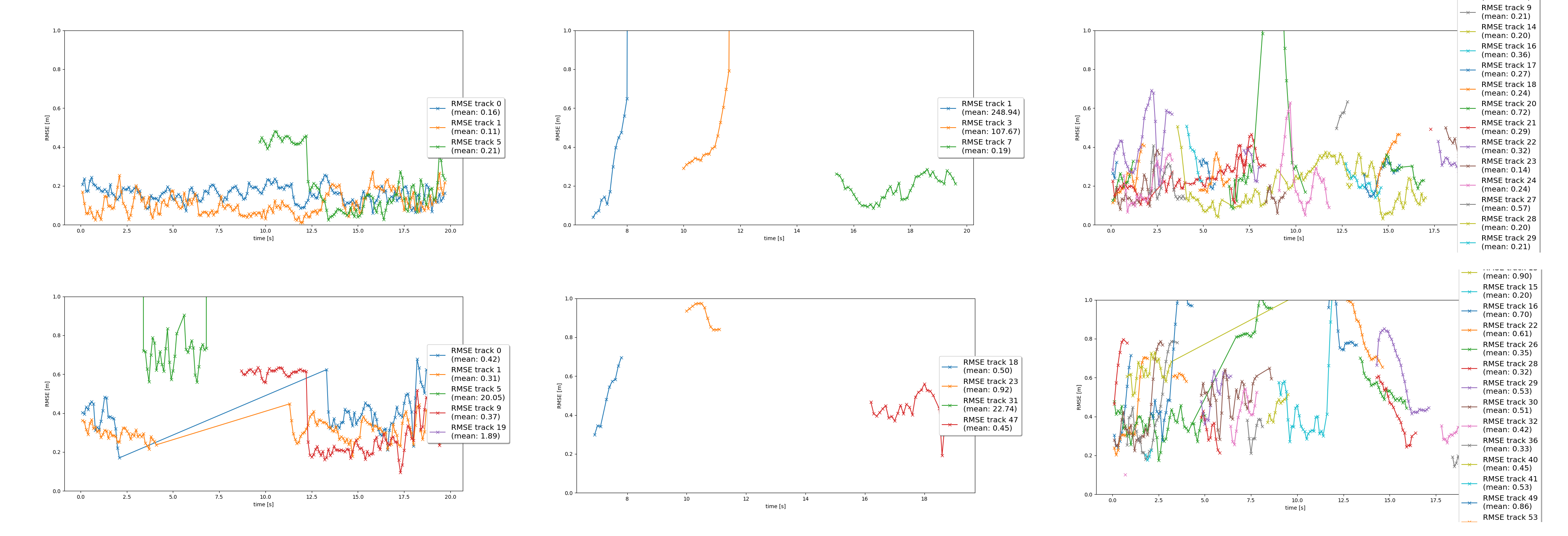
As we can see in the image above a comparison of the results for both models and over each track. Resnet (first row) perform better overall and best in the first track (first column). Despite the high RMSE values in the second track (second column) both models identify and track the main vehicles in the same time range.
Unfortunately, the lack of LiDAR measurements in the precomputed values results in an increase of RMSE.
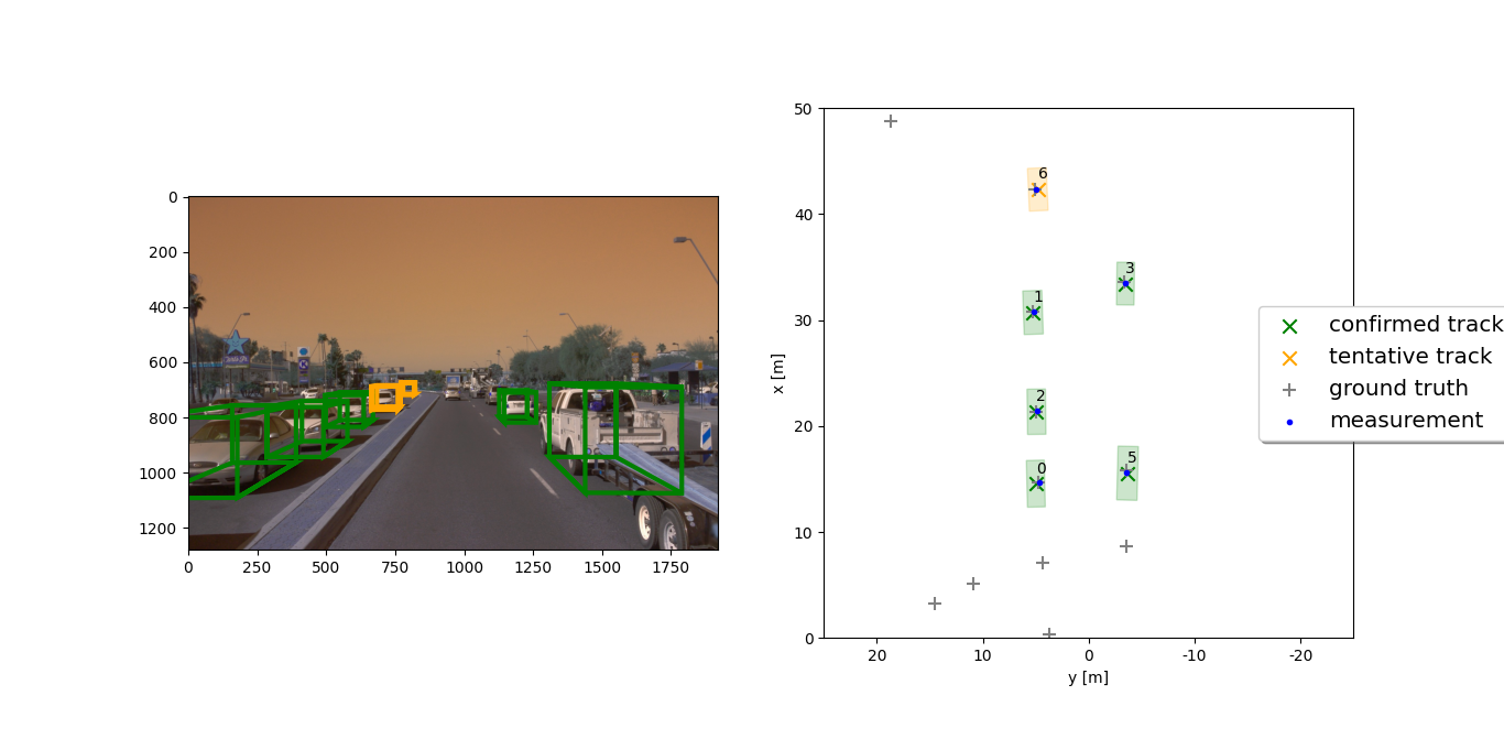
A visualization of the tracking process is displayed below: 6 vehicles are correctly identified in accordance with the LiDAR measurements, 5 of which are confirmed tracks and 1 is tentative (meaning that further calculation are necessary at this stage).
Conclusion
Accurate 3D object detection and tracking are core tasks in state-of-the-art driving systems. Camera images alone lack depth information, making the detection ambiguous. The use of an Extended Kalman Filter to combine a deep learning approach on LiDAR data and RGB camera images improves significantly the accuracy in tracking vehicles over time.
A comparison between Resnet and Darknet was provided using precision and recall as metrics in the object detection step. The results showed that while the object detector using Resnet has a higher precision, Darknet leads to higher recall values. Further studies with different metrics can be done to assert the advantages of one model over the other.
Furthermore, the tracking process was evaluated using RMSE, showing optimal results for the Resnet model in the first track, but suboptimal in the other cases potentially due to inaccuracy of data.
Overall, this represents a starting point with lots of room for future developments. The parametrization process can be fine-tuned to reduce the RMSE during tracking: one idea would be to apply the standard deviation values for LiDAR instead of fixed parameters. Similarly, a more advanced data association (Global Nearest Neighbor (GNN) or Joint Probabilistic Data Association (JPDA)) can be implemented. Since the precomputed detections contain a lot of false negatives (lots of ground truths without measurements) a new detection model could be computed instead.
On the tracking side, the Kalman filter could be adapted to also estimate the object’s width, length, and height, instead of simply using unfiltered lidar detections, in addition to use a non-linear motion model (e.g. a bicycle model) which is more appropriate for vehicle movement than the linear motion model used, since a vehicle can only move forward or backward, not in any direction.
References
[1] Hong-Yuan Mark Liao Alexey Bochkovskiy, Chien-Yao Wang. 2020. YOLOv4: Optimal Speed and Accuracy of Object Detection. arXiv (2020).
[2] Mayank Bansal, Alex Krizhevsky, and Abhijit Ogale. 2018. Chauffeur-Net: Learning to Drive by Imitating the Best and Synthesizing the Worst. arXiv:1812.03079 [cs.RO]
[3] Gioele Ciaparrone, Francisco Luque Sánchez, Siham Tabik, Luigi Troiano, Roberto Tagliaferri, and Francisco Herrera. 2020. Deep learning in video multi-object tracking: A survey. Neurocomputing 381 (2020), 61–88. https://doi.org/10.1016/j. neucom.2019.11.023
[4] Nguyen Mau Dung. 2020.Super-Fast-Accurate-3D-Object-Detection-PyTorch. https://github.com/maudzung/Super-Fast-Accurate-3D-Object-Detection.
[5] Peiyun Hu, Jason Ziglar, David Held, and Deva Ramanan. 2020. What You See is What You Get: Exploiting Visibility for 3D Object Detection. arXiv:1912.04986 [cs.CV]
[6] Roger Labbe. 2014. Kalman and Bayesian Filters in Python. https://github.com/rlabbe/Kalman-and-Bayesian-Filters-in-Python.
[7] Peixuan Li, Huaici Zhao, Pengfei Liu, and Feidao Cao. 2020. RTM3D: Realtime Monocular 3D Detection from Object Keypoints for Autonomous Driving. arXiv:arXiv:2001.03343
[8] Karl Amende-Horst-Michael Gross Martin Simon, Stefan Milz. 2018. Complex-YOLO: Real-time 3D Object Detection on Point Clouds. arXiv (2018).
[9] Pei Sun, Henrik Kretzschmar, Xerxes Dotiwalla, Aurelien Chouard, Vijaysai Patnaik, Paul Tsui, James Guo, Yin Zhou, Yuning Chai, Benjamin Caine, et al. 2020. Scalability in perception for autonomous driving: Waymo open dataset. In Proceedings of the IEEE/CVF Conference on Computer Vision and Pattern Recognition.2446–2454.
[10] Sebastian Thrun, Dieter Fox, Wolfram Burgard, and Frank Dellaert. 2001. Robust Monte Carlo localization for mobile robots. Artificial intelligence 128, 1-2 (2001), 99–141.