Advanced Lane Finding (Code)
The goal of this project is to write a software pipeline to identify the lane boundaries in a video from a front-facing camera on a car. At first the pipeline is developed on a series of individual images, and later the result is applied to a video stream.
The steps followed are:
- Compute the camera calibration matrix and distortion coefficients given a set of chessboard images.
- Apply a distortion correction to raw images.
- Use color transforms and gradients to create a thresholded binary image.
- Apply a perspective transform to rectify binary image (“birds-eye view”).
- Detect lane pixels and fit to find the lane boundary.
- Determine the curvature of the lane and vehicle position with respect to center.
- Warp the detected lane boundaries back onto the original image.
- Output visual display of the lane boundaries and numerical estimation of lane curvature and vehicle position.
The project is developed using Python and OpenCv. You can download the full code from GitHub.
Camera Calibration
I start by initializing object points and imgpoints, the arrays containing respectively the 3D points in real world space and the 2D points in image space.
# Array to store object points and image points from all the images
objpoints = [] # 3D points in real world space
imgpoints = [] # 2D points in images plane

# Prepare object points, like (0,0,0), (1,0,0),...
objp = np.zeros((nx*ny,3), np.float32)
objp[:,:2] = np.mgrid[0:nx,0:ny].T.reshape(-1,2) # x, y coordinates
Here I am assuming the chessboard is fixed on the (x, y) plane at z=0, such that the object points are the same for each calibration image. Thus, objp is just a replicated array of coordinates that will be appended to objpoints every time all chessboard corners are successfully detected in a test image. At the same time, the (x, y) pixel position of each of the corners in the image plane will be appended to imgpoints.
I then used the output objpoints and imgpoints to compute the camera calibration and distortion coefficients using the cv2.calibrateCamera() function.
for fname in images:
    # Read in each image
    img = cv2.imread(fname)

    # Convert to grayscale
    gray = cv2.cvtColor(img, cv2.COLOR_BGR2GRAY)

    # Find the chessboard corners
    ret, corners = cv2.findChessboardCorners(gray, (nx, ny), None)

    # If corners are found, draw corners
    if ret == True:
        imgpoints.append(corners)
        objpoints.append(objp)

# Camera calibration, given object points, image points, and the shape of the grayscale image
ret, mtx, dist, rvecs, tvecs = cv2.calibrateCamera(objpoints, imgpoints, gray.shape[::-1], None, None)
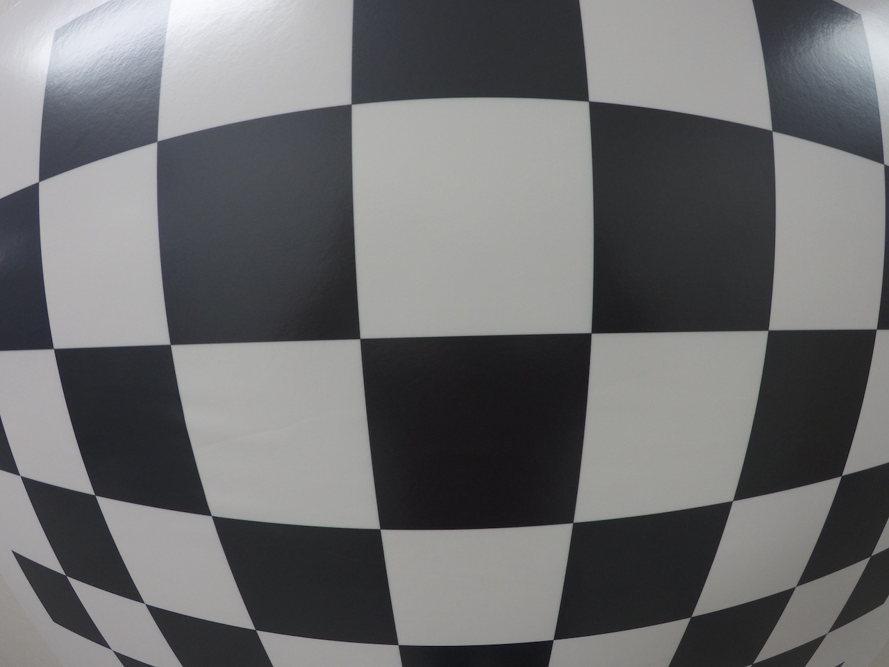
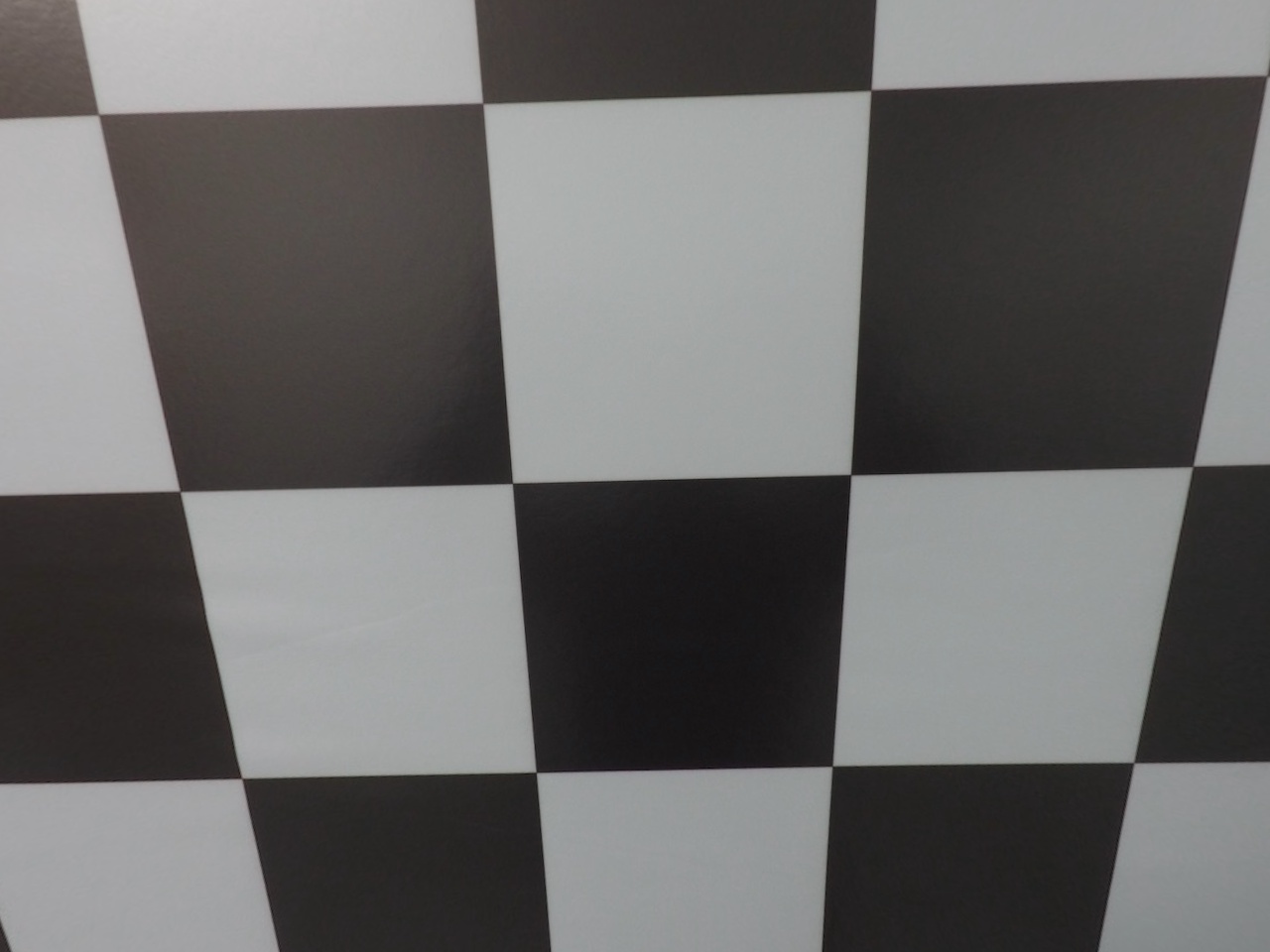
I applied this distortion correction to the test image using the cv2.undistort() function
def distortion_correction(image, mtx, dist):
  dst = cv2.undistort(image, mtx, dist, None, mtx)
  return dst
and obtained this result:
Pipeline
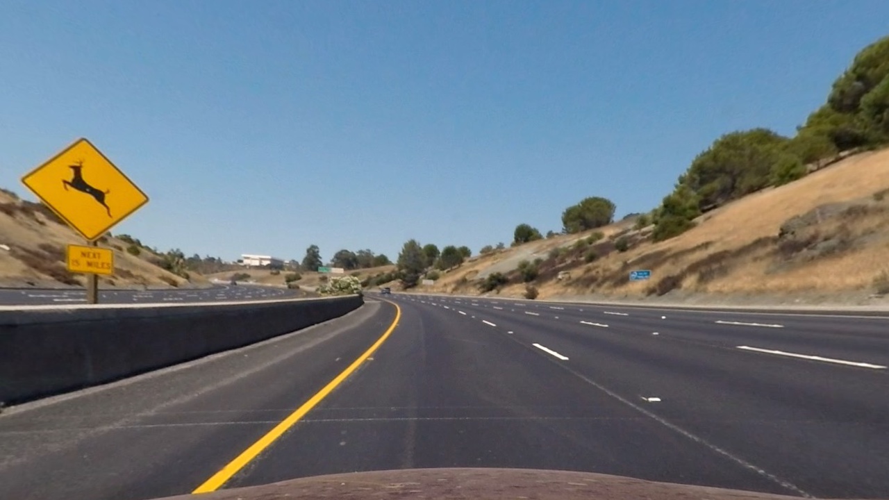
As a first step, I applied the distortion correction to one of the test images:
Then, I used a combination of color and gradient thresholds to generate a binary image:
def color_gradient_transform(img, sobel_size=9, gaussian_kernel=5,
                             grad_thresh=(0, 100), mag_thresh=(0, 100), dir_thresh=(0.7, 1.3),
                             gray_thresh=(0, 100), red_thresh=(0, 100), h_thresh=(0, 100), s_thresh=(0, 100)):

    img = np.copy(img)

    # Gradient transform
    gradient_binary = gradient_transform(img, sobel_size, gaussian_kernel,
                                         grad_thresh=grad_thresh, mag_thresh=mag_thresh, dir_thresh=dir_thresh)

    # Color transform
    color_binary = color_transform(img, gaussian_kernel,
                                   gray_thresh=gray_thresh, red_thresh=red_thresh, h_thresh=h_thresh, s_thresh=s_thresh)

    # Combine the two binary thresholds
    combined_binary = np.zeros_like(gradient_binary)
    combined_binary[(color_binary == 1) | (gradient_binary == 1)] = 1

    return combined_binary

    test_trasf = color_gradient_transform(dist_img, ksize, gaussian_kernel,
                                      grad_thresh=(95, 100), mag_thresh=(95, 100), dir_thresh=(0.7, 1.3),
                                      gray_thresh=(95, 100), red_thresh=(98, 100), h_thresh=(20, 30), s_thresh=(90, 100))
Here’s an example of my output for this step.
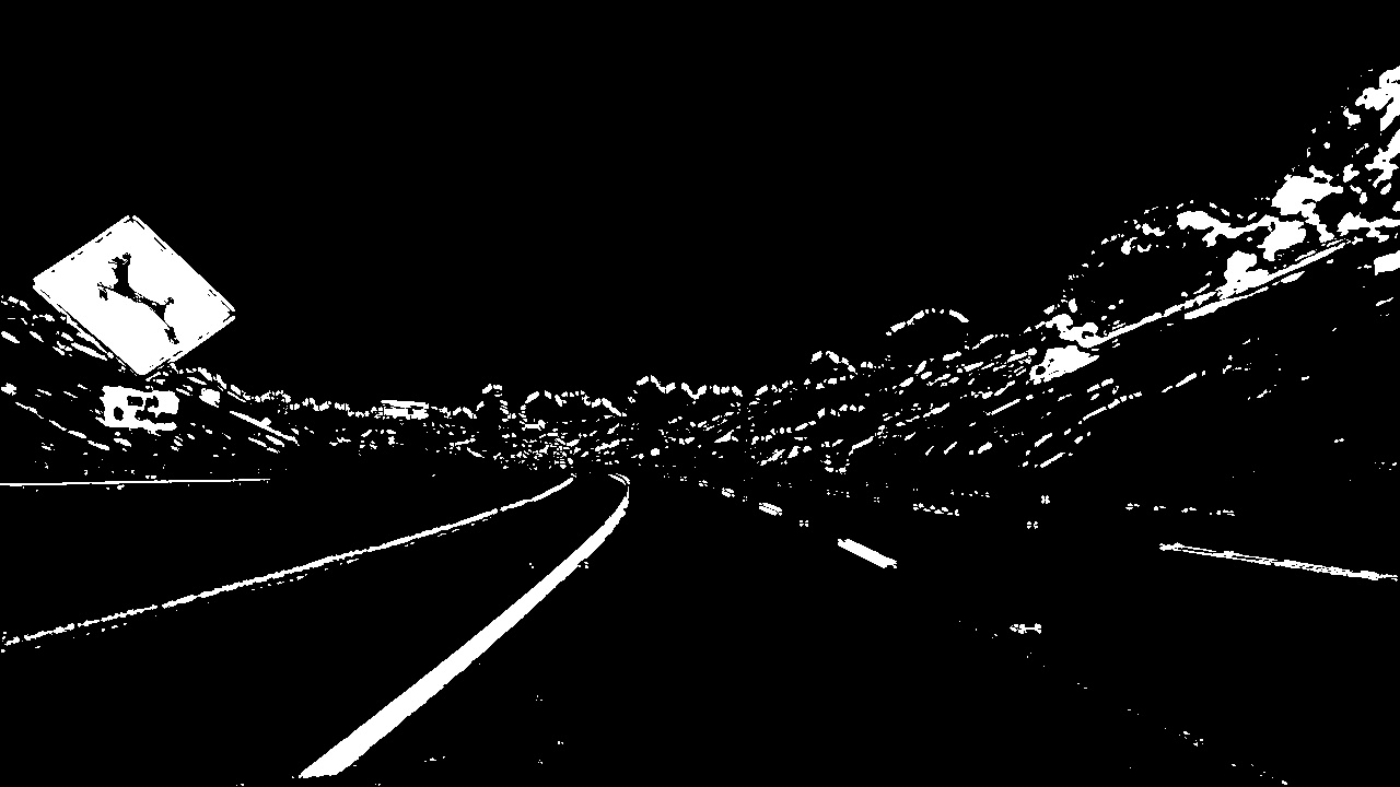
In the color transform I combined grayscale, binary red channel, binary h channel and binary s channel.
def color_transform(img, gaussian_kernel=5, gray_thresh=(95, 100), red_thresh=(98, 100), h_thresh=(30, 50), s_thresh=(90, 100)):

    # Create gray image
    gray_img = gray_binary(img, thresh=gray_thresh)
    blur_gray = cv2.GaussianBlur(gray_img, (gaussian_kernel, gaussian_kernel), 0)
    # Create red image
    red_img = red_binary(img, thresh=red_thresh)

    # Create h channel image
    h_img = h_binary(img, gaussian_kernel=gaussian_kernel, thresh=h_thresh)

    # Create s channel image
    s_img = s_binary(img, gaussian_kernel=gaussian_kernel, thresh=s_thresh)

    combined_binary = np.zeros_like(s_img)
    combined_binary[((gray_img == 1) & (red_img == 1)) | ((h_img == 1) & (s_img == 1))] = 1
#     [((blur_gray == 1) | (red_img == 1)) | ((h_img == 1) | (s_img == 1))] = 1

    return combined_binary
While in the gradient transform I used the gradient along the x and y axis, the magnitude and direction of the gradient.
def gradient_transform(img, sobel_kernel=3, gaussian_kernel=5, grad_thresh=(0, 100), mag_thresh=(0, 100), dir_thresh=(0, np.pi/2)):

    # Create x and y gradients images
    gradx = abs_sobel_thresh(img, orient='x', sobel_kernel=ksize, gaussian_kernel=gaussian_kernel, thresh=grad_thresh)
    grady = abs_sobel_thresh(img, orient='y', sobel_kernel=ksize, gaussian_kernel=gaussian_kernel, thresh=grad_thresh)

    # Create magnitude image
    mag_binary = mag_threshold(img, sobel_kernel=ksize, gaussian_kernel=gaussian_kernel, mag_thresh=mag_thresh)

    # Create gradient direction image
    dir_binary = dir_threshold(img, sobel_kernel=ksize, gaussian_kernel=gaussian_kernel, thresh=dir_thresh)

    combined_binary = np.zeros_like(dir_binary)
    combined_binary[((gradx == 1) & (grady == 1)) | ((mag_binary == 1) & (dir_binary == 1))] = 1

    return combined_binary
It’s important to notice that after grayscaling the image to apply the different thresholds, I used a Gaussian Filter to smooth out the image.
# Convert to grayscale
gray = cv2.cvtColor(img, cv2.COLOR_RGB2GRAY)
# Gaussian Filter
blur_gray = cv2.GaussianBlur(gray, (gaussian_kernel, gaussian_kernel), 0)
And I used percentile thresholding to apply the different thresholds.
# Create percentile-based thresholds
thresh_min = np.percentile(blur_gray, thresh[0])
thresh_max = np.percentile(blur_gray, thresh[1])

# Apply threshold
gray_binary = np.zeros_like(blur_gray)
gray_binary[(blur_gray > thresh_min) & (blur_gray <= thresh_max)] = 1
The code for my perspective transform includes a function called perspective_trasform() where I chose to hardcode the source and destination points in the following manner:
def perspective_trasform(image):

    img_size = (image.shape[1], image.shape[0])

    # Define source points and destination points
    src = np.float32(
        [[(img_size[0] / 2) - 55, img_size[1] / 2 + 100],
        [((img_size[0] / 6) - 10), img_size[1]],
        [(img_size[0] * 5 / 6) + 60, img_size[1]],
        [(img_size[0] / 2 + 55), img_size[1] / 2 + 100]])
    dst = np.float32(
        [[(img_size[0] / 5), 0],
        [(img_size[0] / 5), img_size[1]],
        [(img_size[0] * 3 / 4), img_size[1]],
        [(img_size[0] * 3 / 4), 0]])

    # Given src and dst points, calculate the perspective transform matrix
    M = cv2.getPerspectiveTransform(src, dst)

    # Calculate inverse perspective matrix
    Minv = cv2.getPerspectiveTransform(dst, src)

    # Warp the image using OpenCV warpPerspective()
    warped = cv2.warpPerspective(image, M, img_size, flags=cv2.INTER_LINEAR)

    # Return the resulting image
    return warped, Minv
This resulted in the following source and destination points:
| Source | Destination |
|---|---|
| 585, 460 | 256, 0 |
| 203, 720 | 256, 720 |
| 1127, 720 | 960, 720 |
| 695, 460 | 960, 0 |
I verified that my perspective transform was working as expected by drawing the src and dst points onto a test image and its warped counterpart to verify that the lines appear parallel in the warped image.
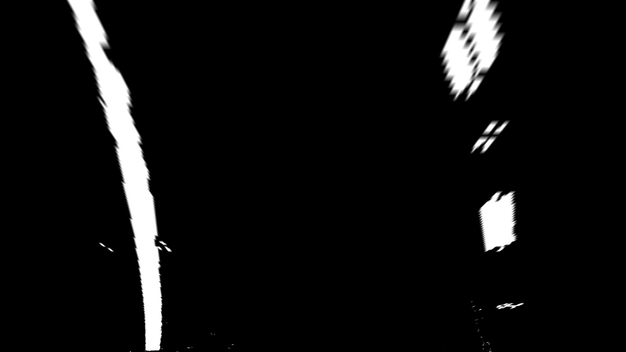
The result of the previous steps is a binary image where the lane lines stand out clearly. However, I have to decide which pixels are part of the lines and which belongs to the left or right lane.
To do so, I first compute the histogram of the peaks of where the binary activations occur across the image.
histogram = np.sum(binary_warped[binary_warped.shape[0]//2:,:], axis=0)
I grab the half bottom of the image [binary_warped.shape[0]//2:,:] because the lanes are most likely to be mostly vertical nearest to the car.
I used a Sliding Window placed around the line centers to find and follow the lines up to the top of the frame.
The 8th cell contains the code I used to detect the lane lines.
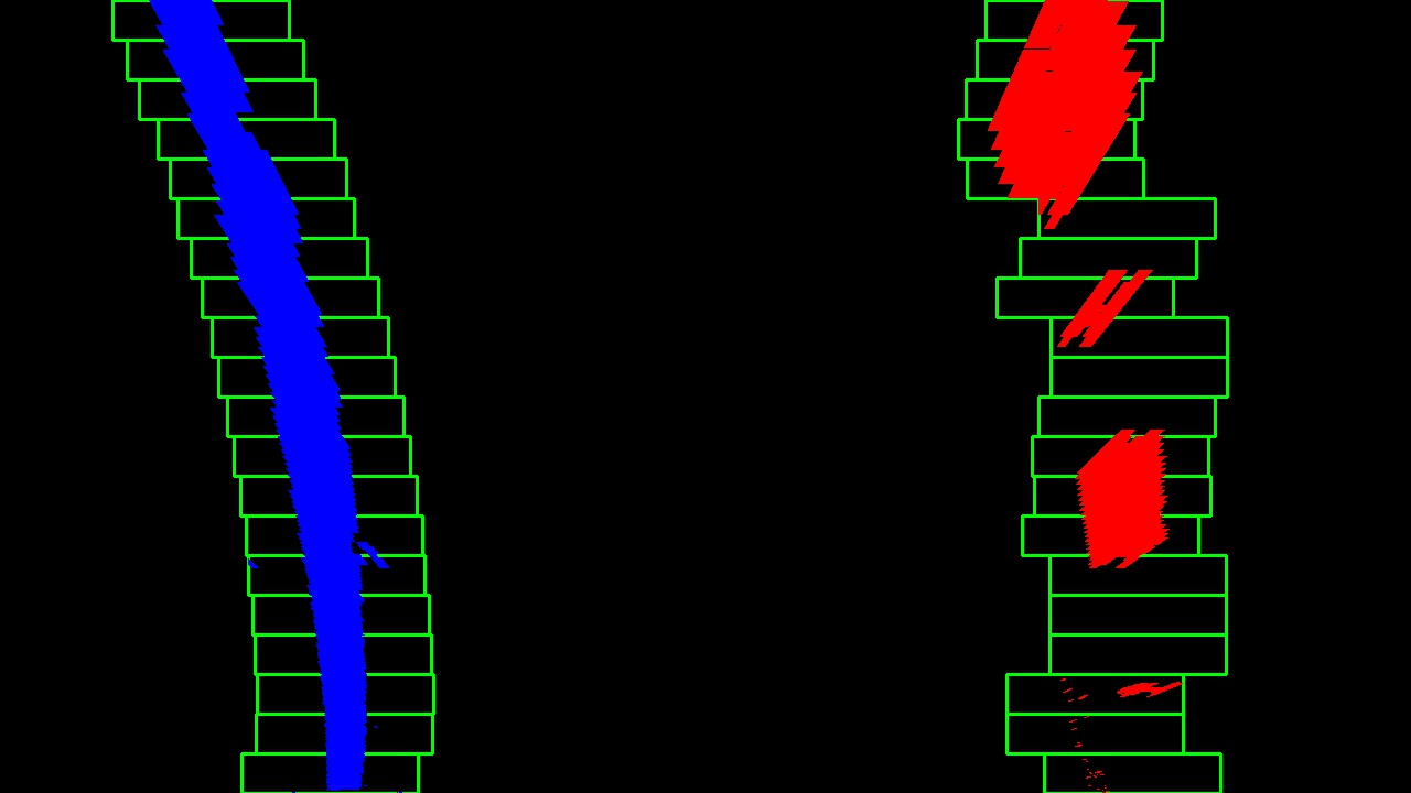
One extra step when the pipeline is performed on a video includes searching for the lane line within a margin around the previous position. This is necessary because using the full algorithm from before and starting fresh on every frame is inefficient, as the lines don’t move a lot from frame to frame.
def search_around_poly(binary_warped, left_lane, right_lane):

    # HYPERPARAMETER
    margin = 100

    # Retrieve lanes previous fit
    prev_left_fit, prev_right_fit = left_lane.best_fit, right_lane.best_fit

    # Grab activated pixels
    nonzero = binary_warped.nonzero()
    nonzeroy = np.array(nonzero[0])
    nonzerox = np.array(nonzero[1])

    ### Set the area of search based on activated x-values ###
    ### within the +/- margin of our polynomial function ###
    left_lane_inds = ((nonzerox > (prev_left_fit[0]*(nonzeroy**2) + prev_left_fit[1]*nonzeroy +
                    prev_left_fit[2] - margin)) & (nonzerox < (prev_left_fit[0]*(nonzeroy**2) +
                    prev_left_fit[1]*nonzeroy + prev_left_fit[2] + margin)))
    right_lane_inds = ((nonzerox > (prev_right_fit[0]*(nonzeroy**2) + prev_right_fit[1]*nonzeroy +
                    prev_right_fit[2] - margin)) & (nonzerox < (prev_right_fit[0]*(nonzeroy**2) +
                    prev_right_fit[1]*nonzeroy + prev_right_fit[2] + margin)))

    # Again, extract left and right line pixel positions
    leftx = nonzerox[left_lane_inds]
    lefty = nonzeroy[left_lane_inds]
    rightx = nonzerox[right_lane_inds]
    righty = nonzeroy[right_lane_inds]

    return leftx, lefty, rightx, righty
``

Next, I measured the radius of curvature:

```python
def measure_curvature_real(ploty, left_fit_cr, right_fit_cr):
    '''
    Calculates the curvature of polynomial functions in meters.
    '''
    # Define conversions in x and y from pixels space to meters
    ym_per_pix = 30/720 # meters per pixel in y dimension
    xm_per_pix = 3.7/700 # meters per pixel in x dimension

    # Define y-value where we want radius of curvature
    # We'll choose the maximum y-value, corresponding to the bottom of the image
    y_eval = np.max(ploty)

    # Calculate the radius of curvature in meters for both lane lines. Should see values of ~1000
    left_curverad = ((1 + (2*left_fit_cr[0]*y_eval*ym_per_pix + left_fit_cr[1])**2)**1.5) / np.absolute(2*left_fit_cr[0])
    right_curverad = ((1 + (2*right_fit_cr[0]*y_eval*ym_per_pix + right_fit_cr[1])**2)**1.5) / np.absolute(2*right_fit_cr[0])

    return left_curverad, right_curverad
The parameters to convert from pixels to meters are based on the assumption that the lane is about 30 meters long and 3.7 meters wide. The final radius is given as the average between the right and left lane radius.
Here is an example of the final result on the test image:

Results
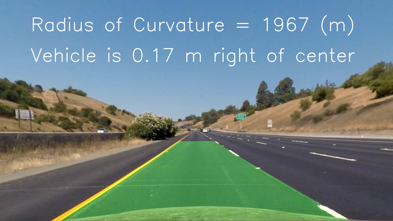
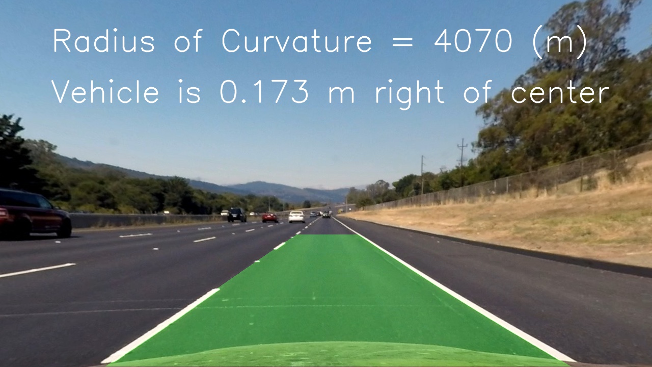
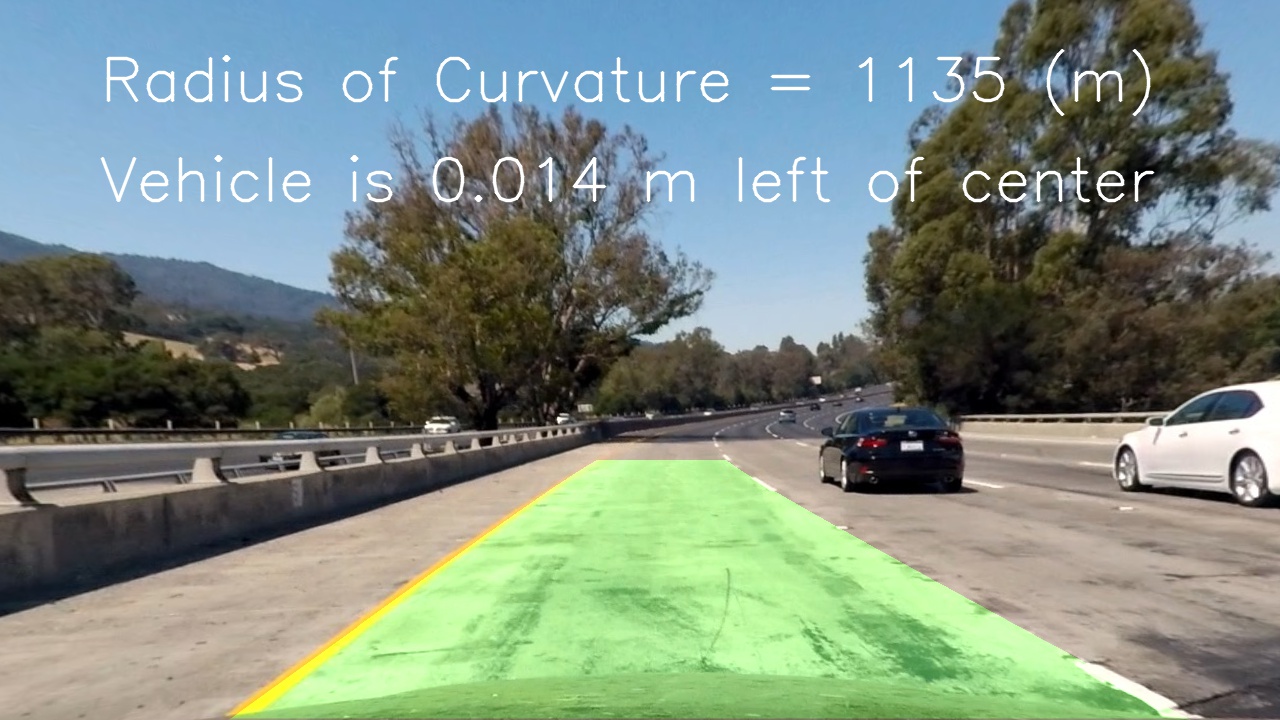
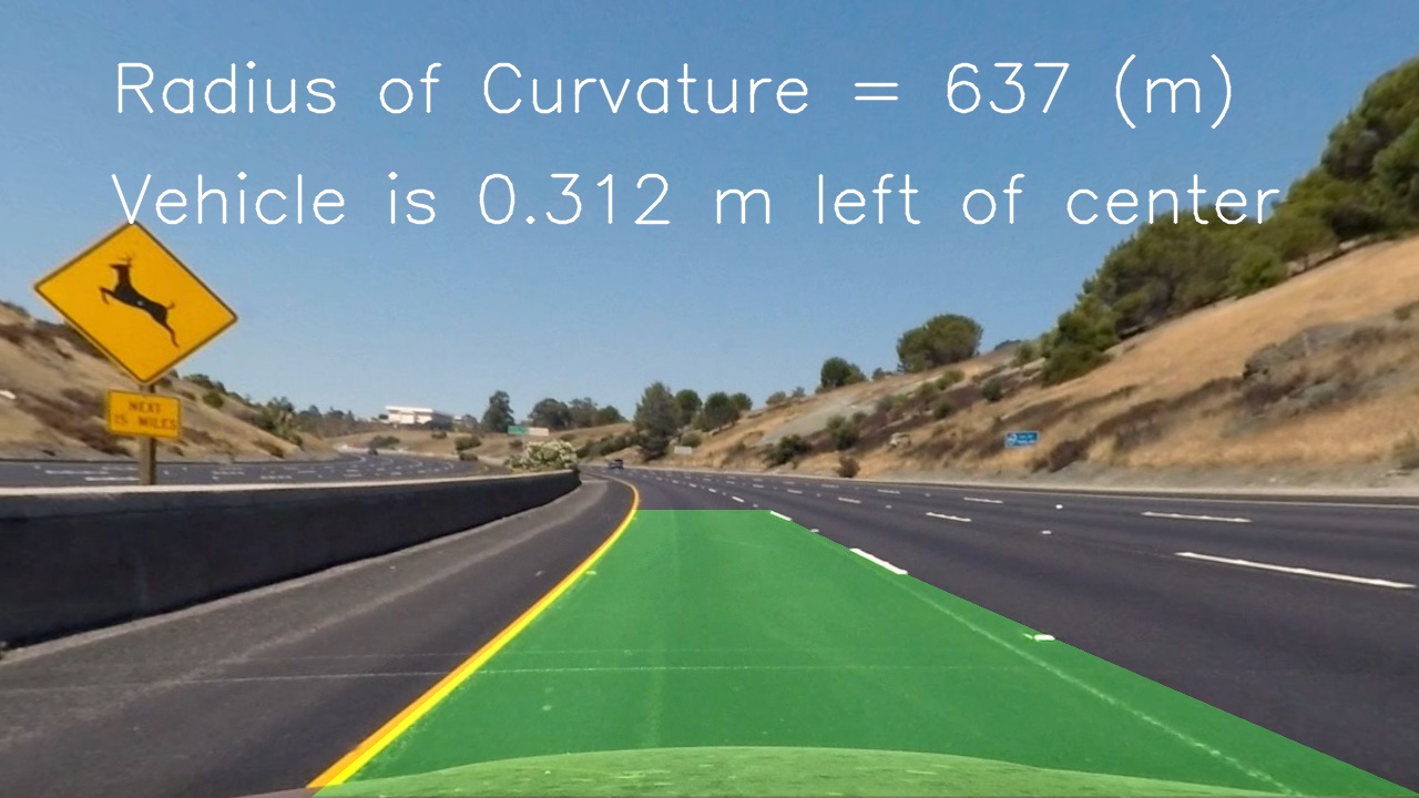
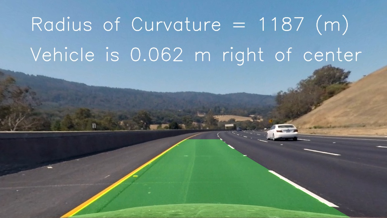
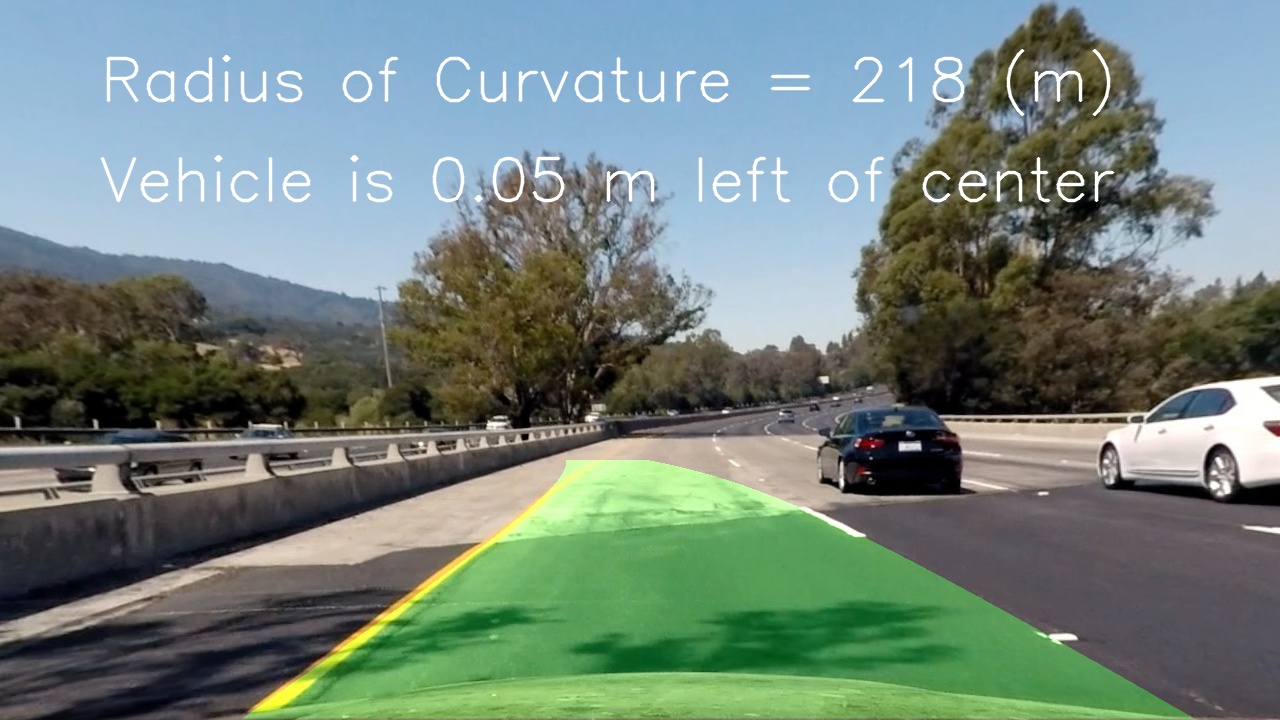
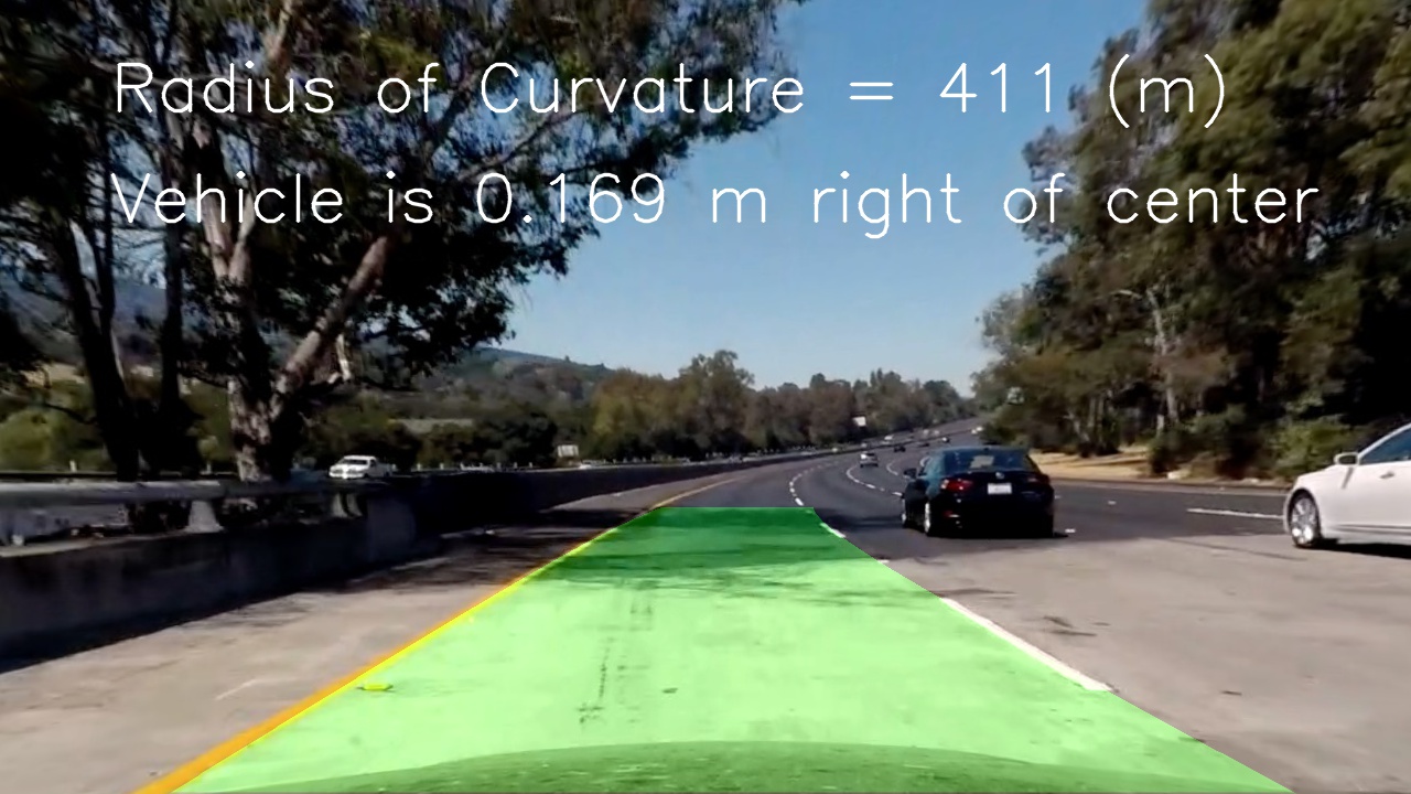
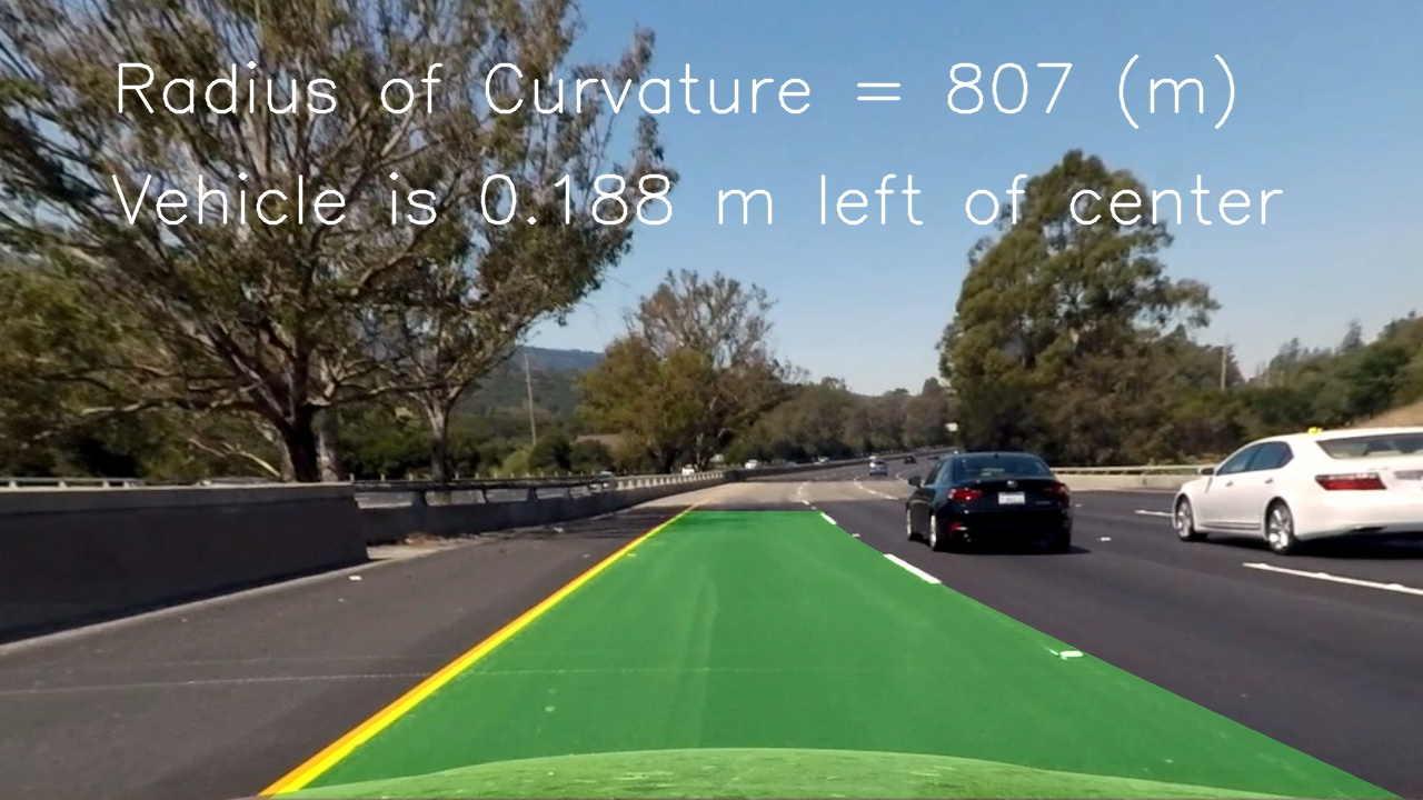
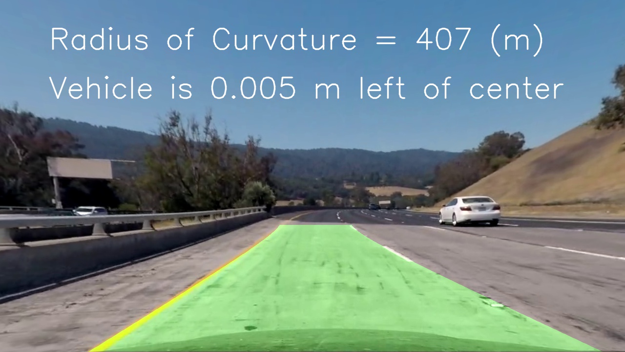
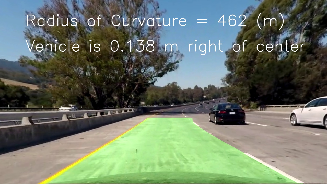
Here’s the result of the pipeline applied to all the test images included in the project:
And the final video:
Shortcomings
One shortcoming occurs when the model doesn’t detect one of the two lines in the first frame.
As an improvement smoothing could be applied to avoid that line detection jumps around from frame to frame.