Advanced Lane Finding
The purpose of this post is to explain the theory behind the project Advanced Lane Finding and build up some intuition about the process. There won’t be any snippets from the source code since we only want to build a high level understanding of why we do what we do.
Computer Vision is the science of perceiving the world around us through images and it plays a major role in helping vehicles move around and navigate safely.
Our goal this time is to write a more sophisticated lane finding algorithm that deals with complex scenarios like curving lines and shadows. We want to measure some of the quantities that we need to know in order to control the car: how much the lanes are curving (useful when you want to steer a car) or where our vehicle is located with respect to the center of the lane.
Distortion Correction
Cameras don’t create perfect images, some of the objects in the images - especially the ones near the edges - can get stretched or skewed and we have to correct for that. But, why does that happen?
Image distortion occurs when a camera looks at 3D objects in the real world and transforms them into a 2D image. When light rays pass through the camera lenses they bend at the edges and this creates an effect that distorts the edges of images, so that lines or objects appear more or less curved than they actually are. This is called radial distortion.
Another type of distortion, is tangential distortion, which occurs when a camera lens is not aligned perfectly parallel to the imaging plane with the result that an image looks tilted.
Distortion changes what the shape and size of these 3D objects appear to be.
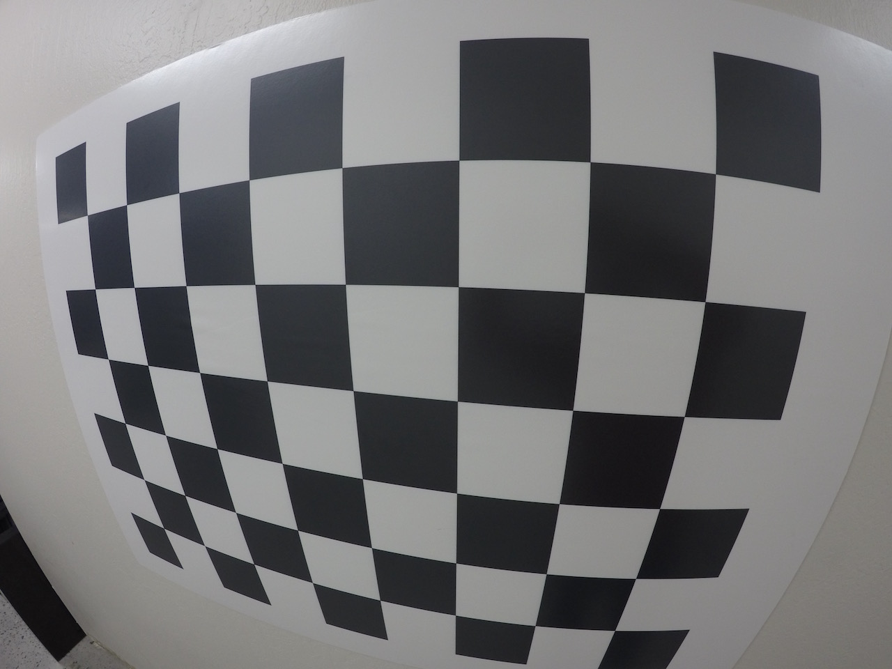
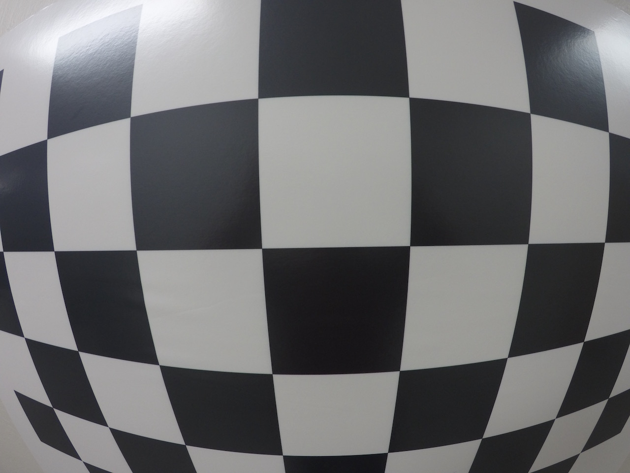
In these distorted images, we can see that the edges of the chessboard are bent and stretched out. This is a problem because to steer a vehicle we need to know how much the lane is curving, and if the image is distorted we’ll get the wrong measure of curvature and our steering angle will be wrong.
So, the first step in analyzing camera images, is to undo this distortion so that we can get correct and useful information out of them.
To undistort the images we’re going to use the equations:

Camera Calibration
We know that distortion changes shape and size of objects in an image. How do we calibrate for that?
We basically take pictures of known shapes so we can detect and correct any distortion error. What shapes are we going to use? A chessboard. That’s because its regular high contrast pattern makes it easy to detect automatically, and we know what an undistorted chessboard looks like.
So, we take multiple pictures of our chessboard against a flat surface
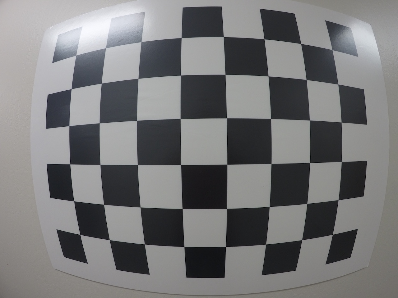
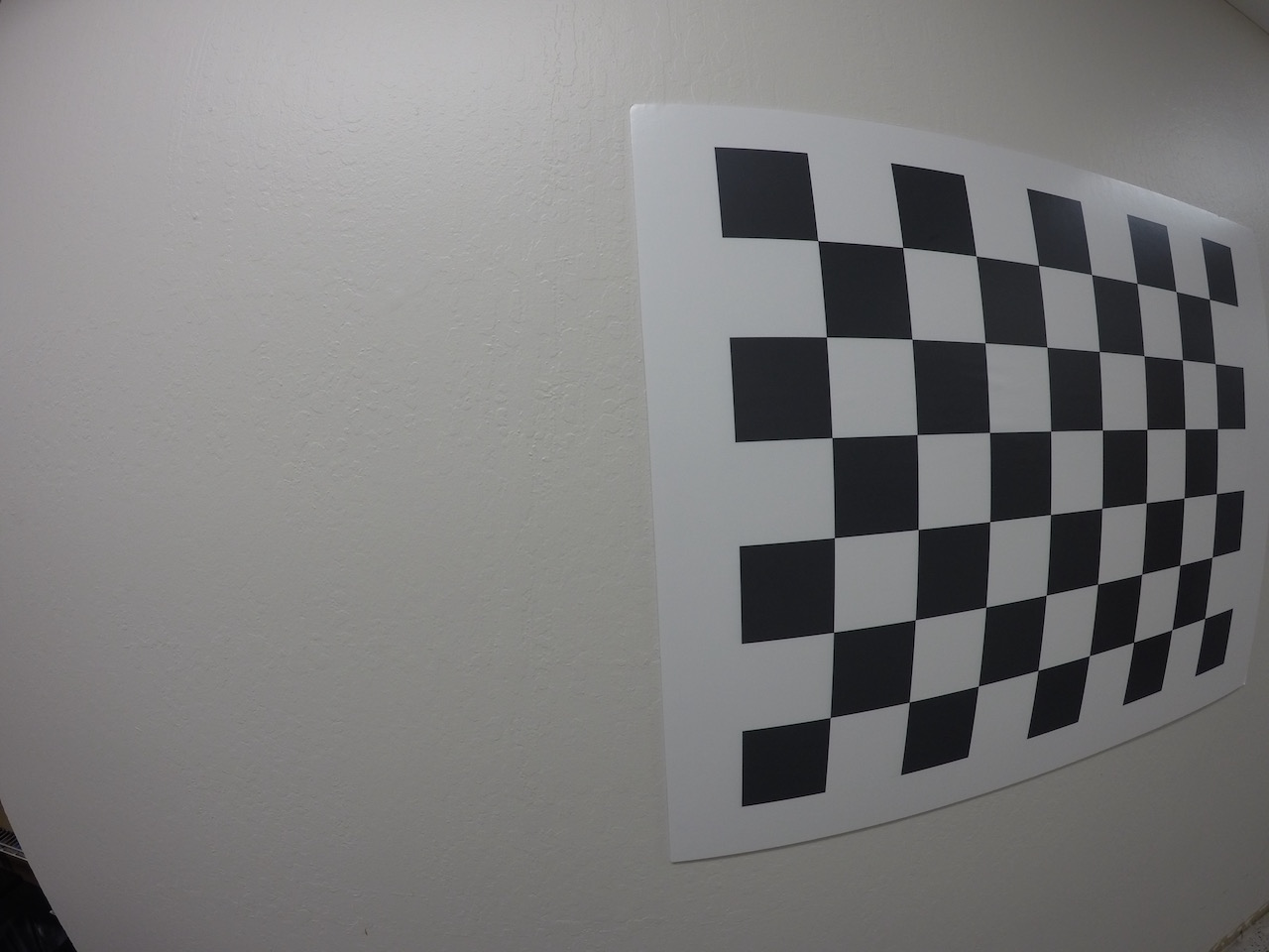
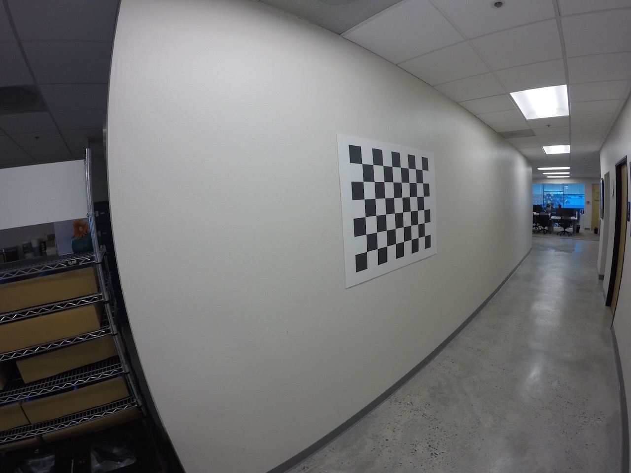
This way, we’ll be able to detect any distortion by looking at the difference between the size and shape of these squares in these images and the size and shape that they actually are. We then create a transform that maps these distorted points to undistorted points to correct any images.
It’s recommended to use at least 20 images to obtain a reliable calibration and it’s useful to notice that we only need to compute it once, and then apply it to undistort each new frame.
Lane Curvature and Vehicle Position
Great! Now, we prepared our images. Let’s keep in mind what our goal is: detect lane lines, measure their curvature and the vehicle position with respect to the center.
We can start by tackling the problem of extracting one really important piece of information from our images: the lane curvature. This is important because to steer a car we need to know how much the lane is curving (together with the speed and dynamics of the car).
To calculate the curvature of a lane line, we’re going to fit a 2nd degree polynomial to that line. For a lane line that is close to vertical, we can fit a line using this formula:
where A gives us the curvature we’re looking for, B gives us the direction that the line is pointing towards, and C gives us the position of the line based on how far away it is from the left side of the image (y = 0).
To find the radius of curvature of the lanes we’re going to use the formula:
Gradient Transform
We know what we need, but how are we going to find it? We’ll be using something called Perspective Transform, but before that there are a couple of image preprocessing steps that we will take to make our job easier: we’ll use color and gradient transforms to create a thresholded binary image.
In the previous project Finding Lane Lines on the Road we used the Canny Edge Detector to find pixels that were likely to be part of a line in an image. This algorithm is great to find all possible lines, but for lane detection it gives us a lot of edges from scenery and cars that we ended up discarding.
To speed up the process we can take advantage of the fact that the lane lines tend to be close to vertical. How can we take advantage of it? We can use gradients only to find steep edges that are more likely to be lanes in the first place.
One operator used to calculate x and y gradients is the Sobel Operator, and if we applied it on an image and took the absolute value:
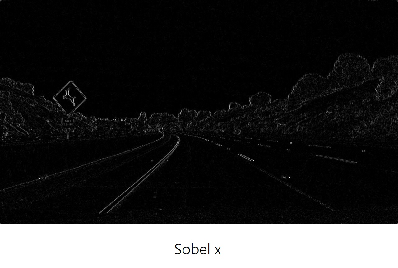
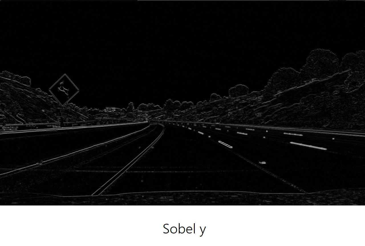
we could see that the gradients taken in both the x and y directions detect the lane lines and pick up other edges. Taking the gradient in the x direction emphasizes edges closer to vertical while the gradient in the y direction emphasizes edges closer to horizontal.
The x-gradient does a cleaner job of picking up the lane lines, but we can see the lines in the y-gradient as well. Given the results, it’s worth exploring other properties of the gradient like magnitude and direction:
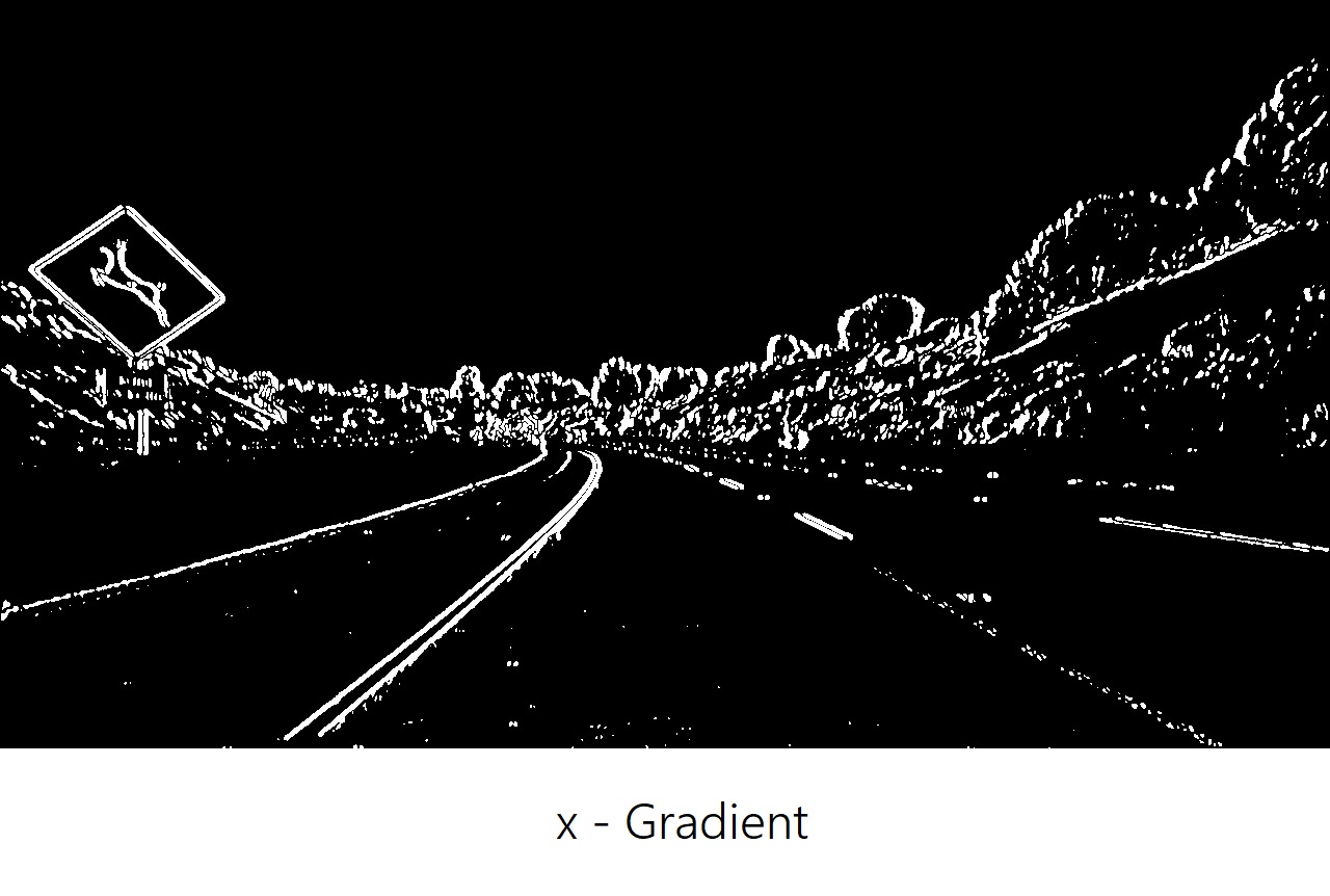
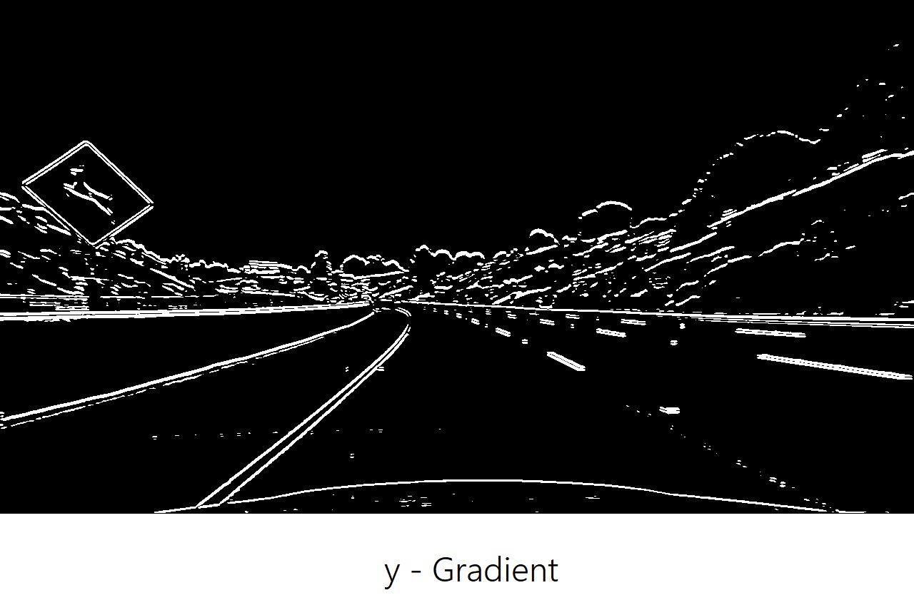
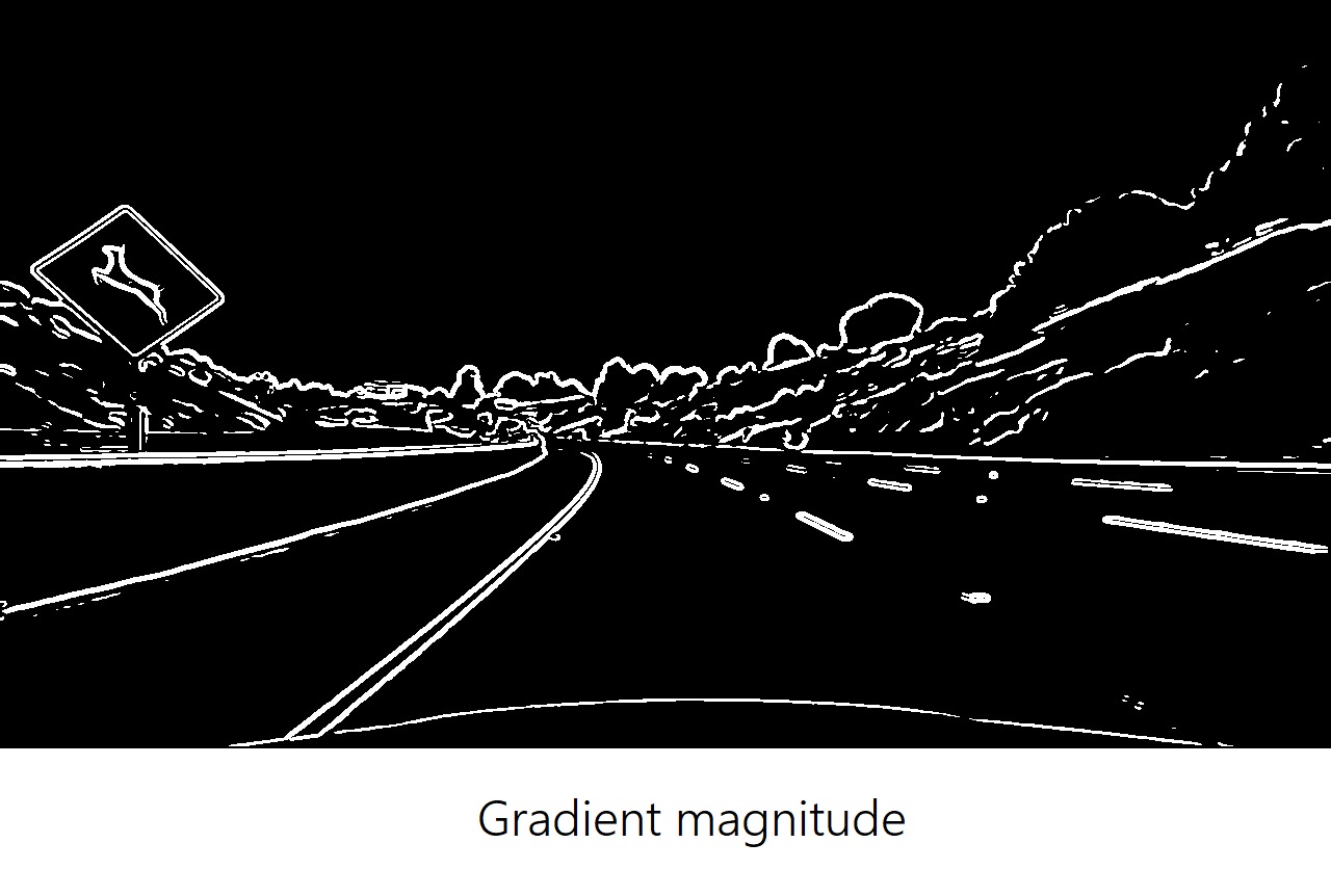
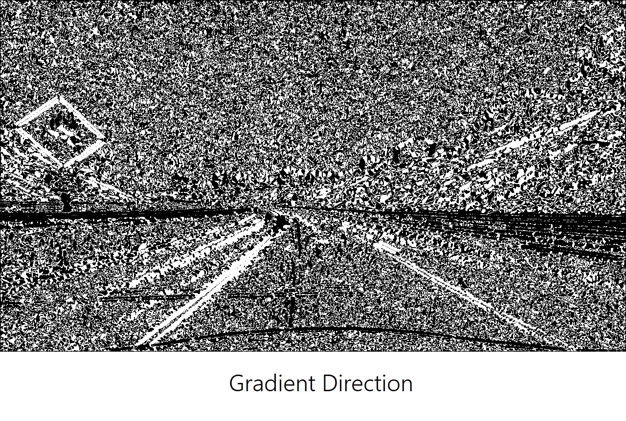
While all these properties are able to identify lane lines, it’s by combining them all together that we obtain the most out of them to isolate lane-line pixels.
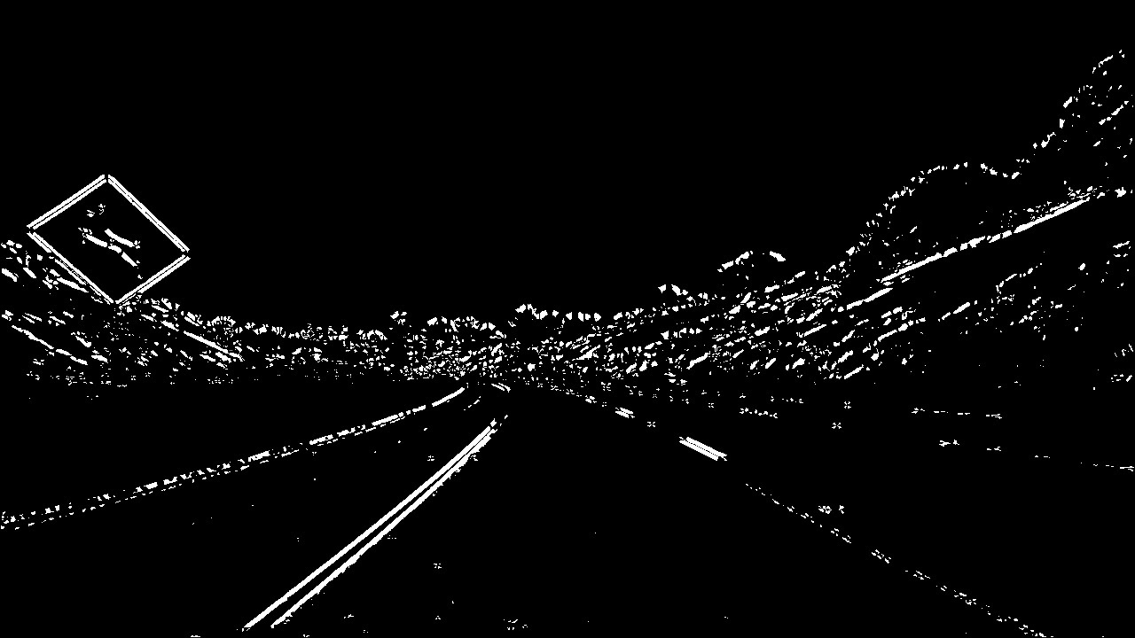
It’s worth noticing that we can modify the kernel size for the Sobel Operator to change the size of this region. Taking the gradient over larger regions can smooth over noisy intensity fluctuations on small scales.
As a general rule, the kernel size should be an odd number. Since we are searching for the gradient around a given pixel, we want to have an equal number of pixels in each direction of the region from this central pixel, leading to an odd-numbered filter size.
Color Transform
When we apply the steps above, one crucial part is converting the image to grayscale. By doing so, we lose some valuable information:
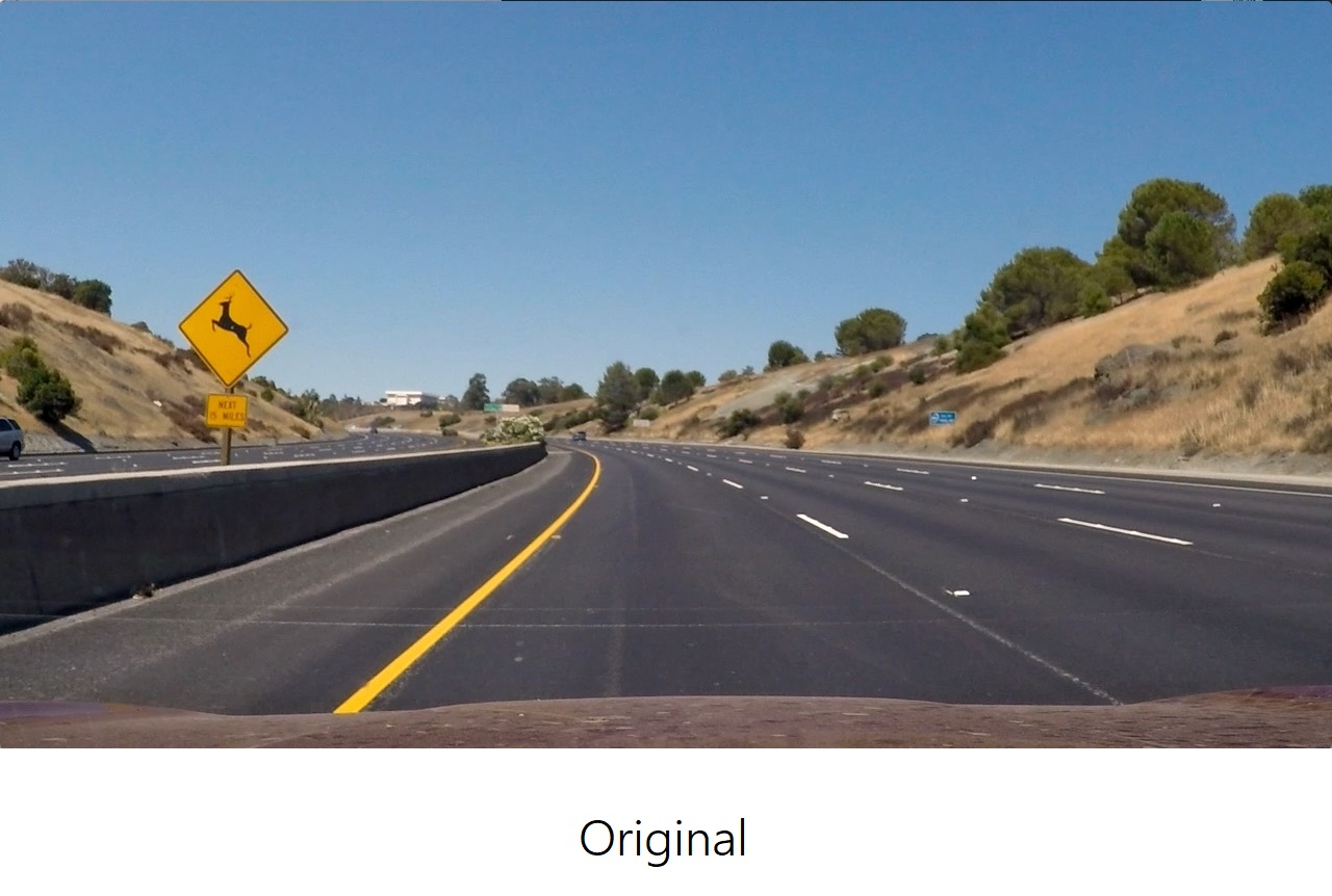
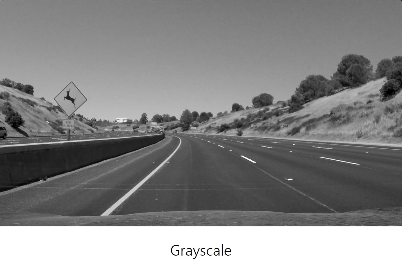
In the grayscale image the yellow line on the left is barely visible, while in the s channel it’s way more clear.
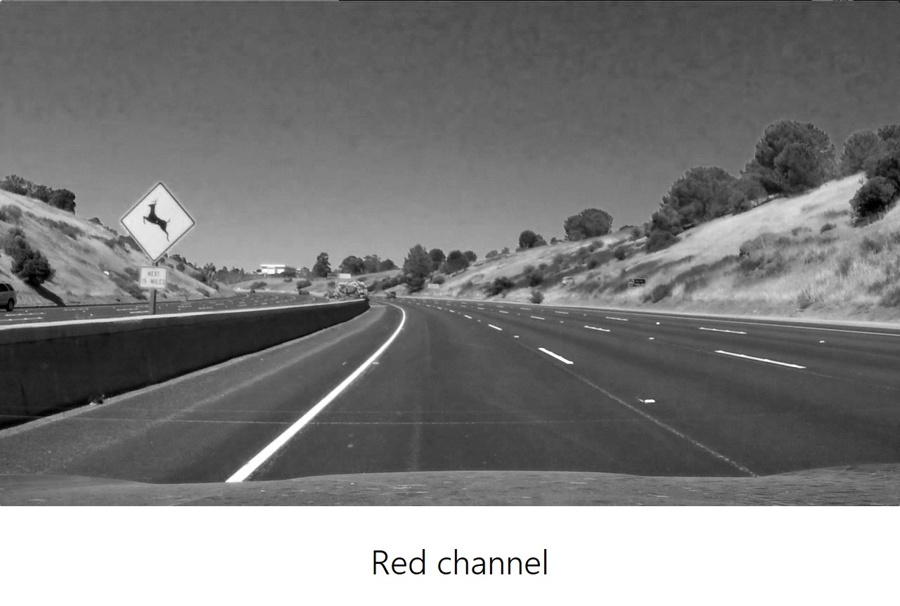
We know that an image is composed of red, blue and green channels. Why can’t we use one of these channels to obtain more information? Let’s take a look at them:

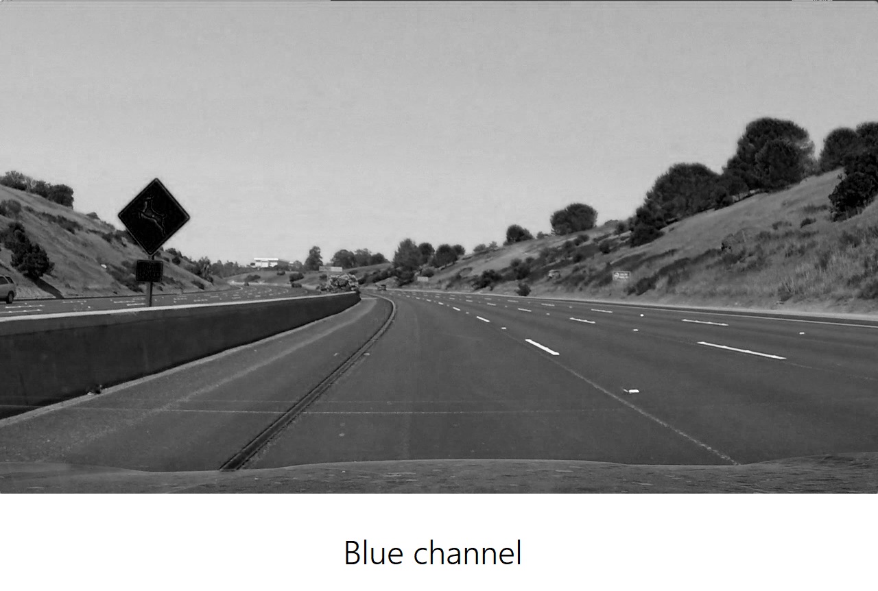
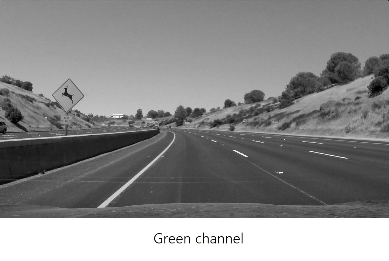
The brighter pixels indicate higher value of the respective channel color.
Looking at the lane lines we can see that the R and G channels are high for both the white and yellow lane line, while the B channel doesn’t detect the yellow lane - there is no blue component in it.
This means that the R and G channels are the most useful to isolate both the white and yellow lane lines. Are we done? No. If we take a closer look at those images we can see that both red and green values change under different levels of brightness at the back of the image, they get lower under shadow and don’t consistently recognize the lane under extreme brightness.
Is there a better way to detect these lanes then? Of course, there are many other ways to represent the color in an image besides RGB channels.
The HLS Color Space, for instance, isolates the lightness (L) component of each pixel in an image. This is the component that varies the most under varies light conditions, while the H and S channels stay consistent in shadow or excessive brightness. So, by using the last two channels only and discard the information in the L channel we’ll be able to detect different colors of lane lines more reliably than in an RGB Space:
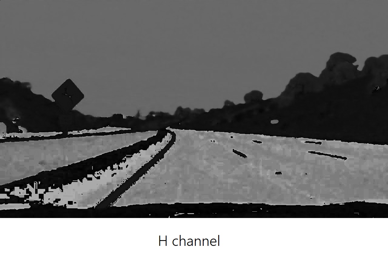
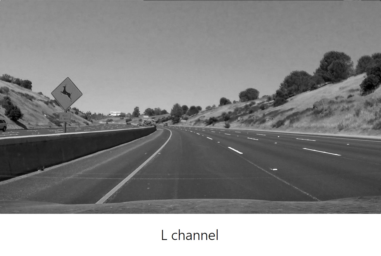
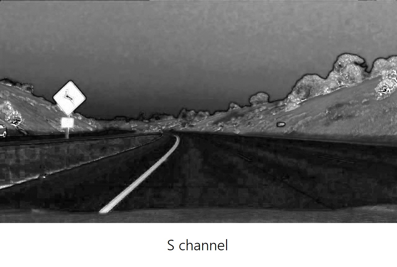
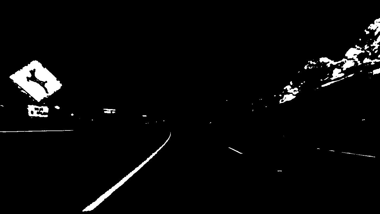
It looks like the S channel detects lane lines pretty well, as well as the dark section of the H channel. Let’s try and compare all these channels to create a color threshold that detects lane line pixels of different colors:
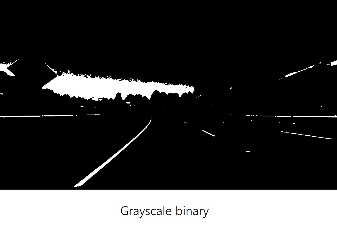
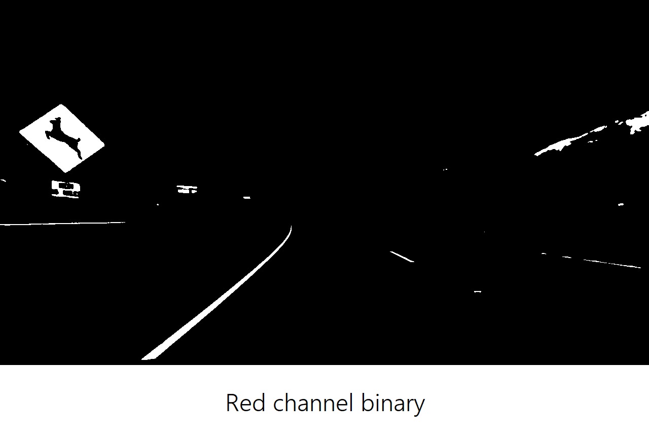
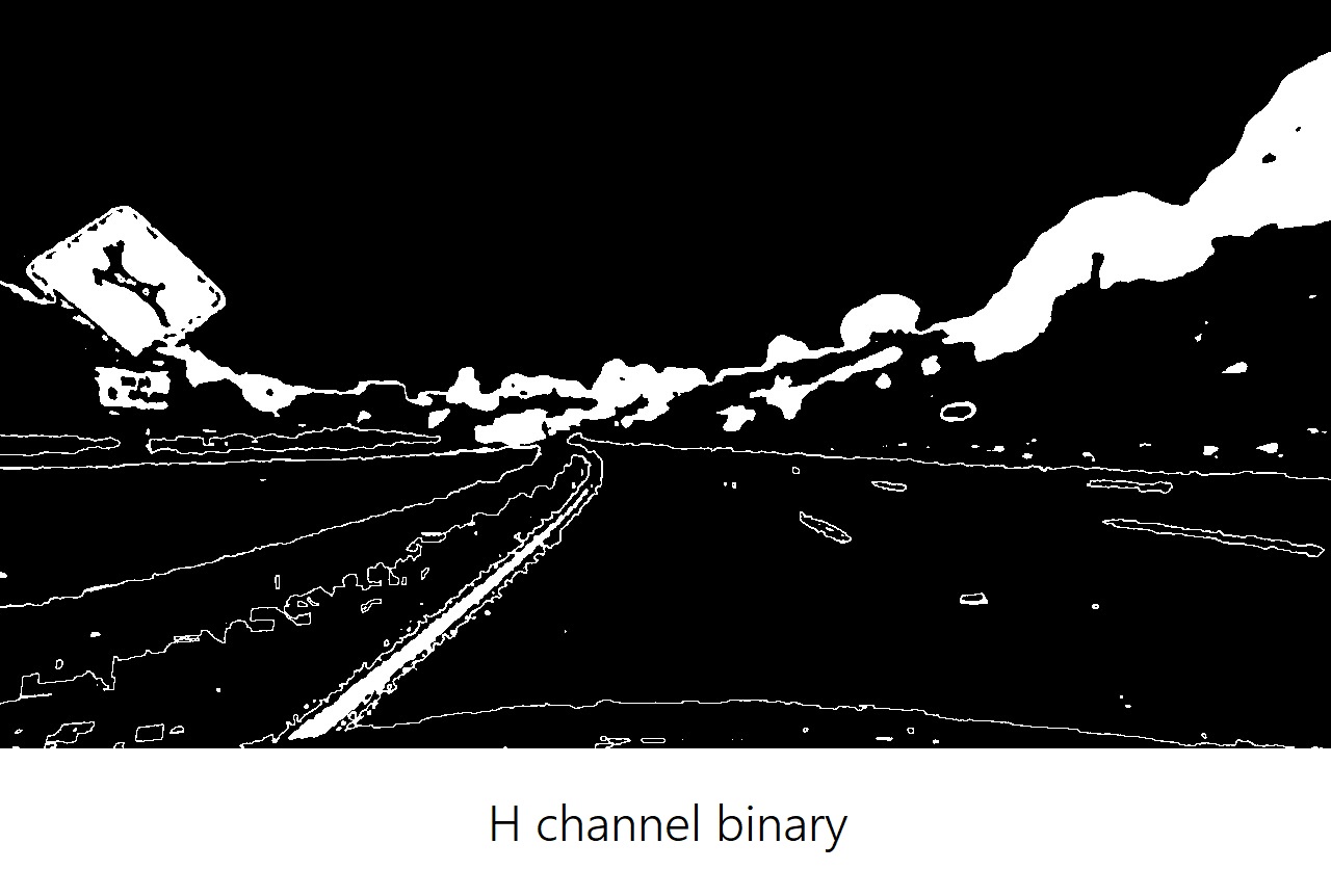
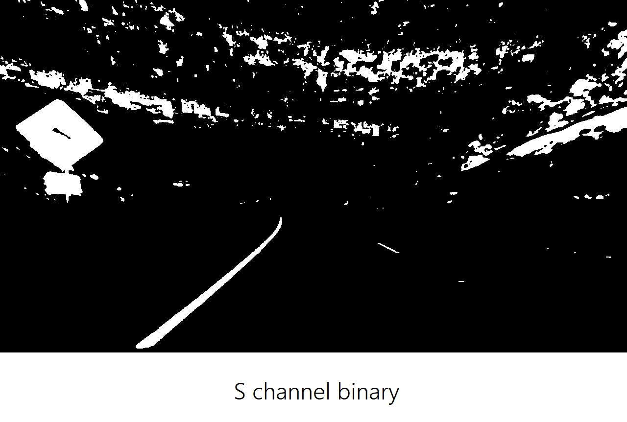
From these examples, we can see that the S channel is doing a robust job of picking up the lines under very different color and contrast conditions. The S channel is cleaner than the H channel and a bit better than the R channel or simple grayscaling. But it’s not clear that one method is far superior to the others.
As with gradients, it’s worth combining various color thresholds to make the most robust identification of the lines.
Color and Gradient Combined
It’s time to combine what we know about color and gradient thresholding to get the best of both worlds.
At this point, it’s okay to detect edges around trees or cars because these lines can be mostly filtered out by applying a mask to the image and cropping out the area outside of the lane lines.
We can see which parts of the lane lines were detected by the gradient threshold and which parts were detected by the color threshold by stacking the channels and seeing the individual components:
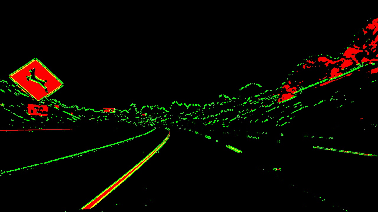
The green is the gradient threshold component and the red is the color channel threshold component.
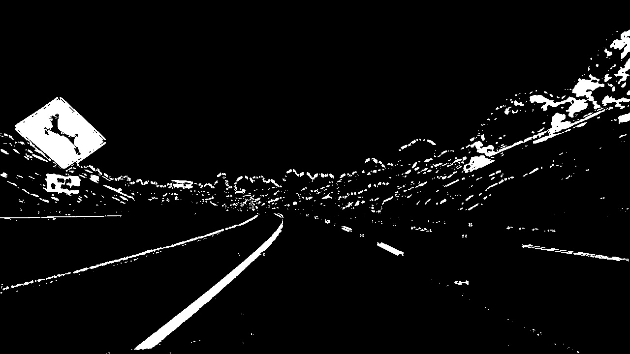
The final black and white combined thresholded image looks like this:
Perspective Transform
A Perspective Transform maps the points in a given image to different image points with a new perspective.
It essentially warps the image by dragging points towards or away from the camera to change the apparent perspective.
Why are we interested in doing a Perspective Transform? Because in reality road boundaries are parallel to each other while in the 2D perspective view they seem to converge to a common point. The perspective projection effect has distorted the shape of the actual road boundaries. Since we ultimately want to measure the curvature of the lines we need to transform to a top-down view, that’s when our lane lines will look parallel and we will be able to fit them with the formula above.

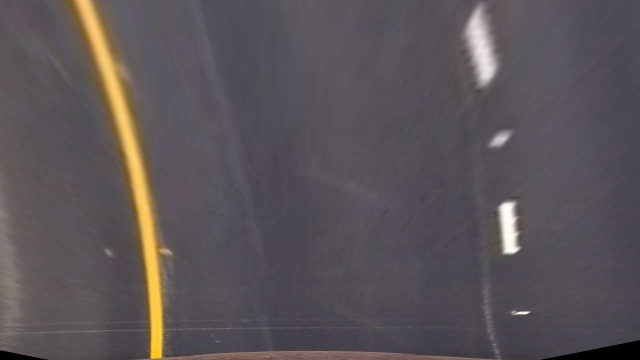
The process of applying a perspective transform is similar to what we did to correct image distortion, but this time we want to map the points in our image to different desired image points with a new perspective.
We are assuming the road is a flat plane. While this isn’t strictly true, it can serve as an approximation in this case.

When applying the transform to new images - to check whether or not we got the transform correct - the lane lines should appear parallel in the warped images whether they are straight or curved.
Since we’re going to apply the Perspective Transform to thresholded binary images, here’s the final result we want to obtain and that will be the starting point for our next step:
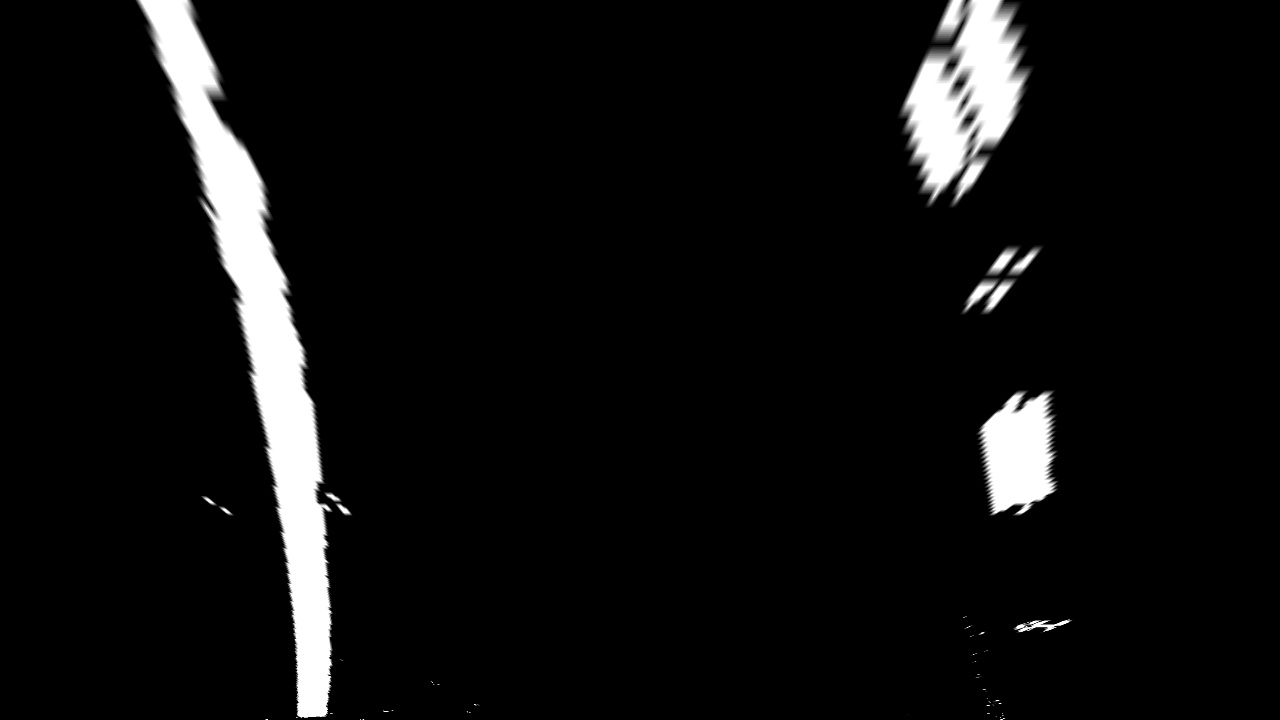
Doing a bird’s eye-view transform is especially useful in this case because it will allow us to match our car location with a map.
Find Lane Boundary
Our ultimate goal was to measure how much the lanes are curving or where our vehicle is located with respect to the center of the lane. We’re almost there.
After applying calibration, thresholding, and a perspective transform to a road image, we have a binary warped image where the lane lines stand out clearly. However, we still need to decide explicitly which pixels are part of the lines and which belong to the left line or the right line.
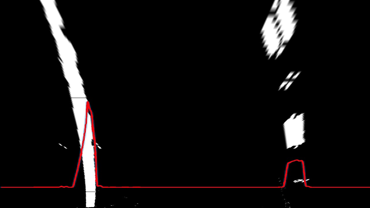
How are we gonna do this? We take a histogram along all the columns in the lower half of the image. Why the lower half? Because the lanes are more likely to be mostly vertical closer to the car.
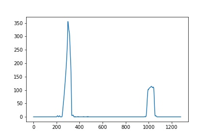
With this histogram we are adding up the pixel values along each column in the image. In our thresholded binary image, pixels are either 0 or 1, so the two most prominent peaks in this histogram will be indicators of the x-position of the base of the lane lines. We can use that as a starting point for where to search for the lines.
From that point, we can use a sliding window - placed around the line centers - to find and follow the lines up to the top of the frame.
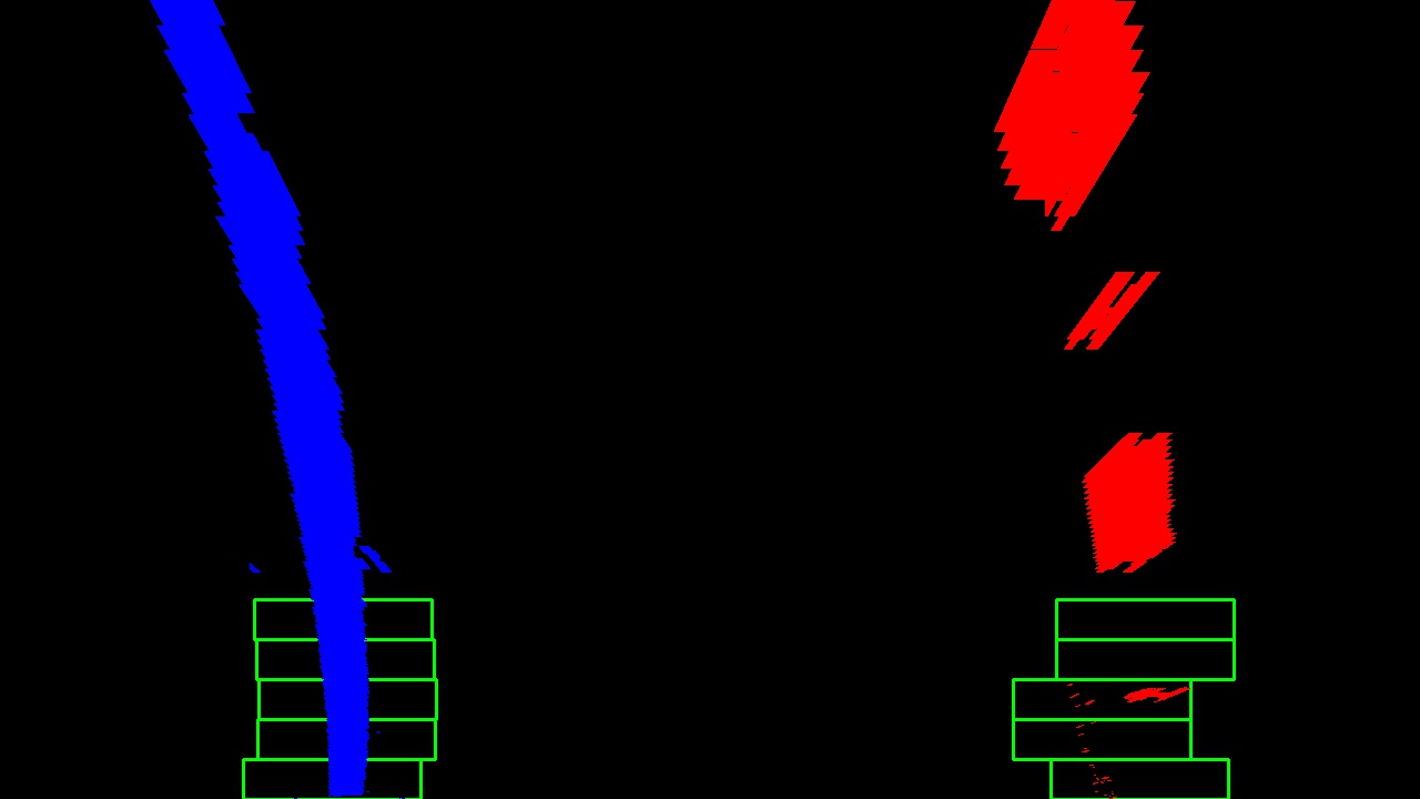
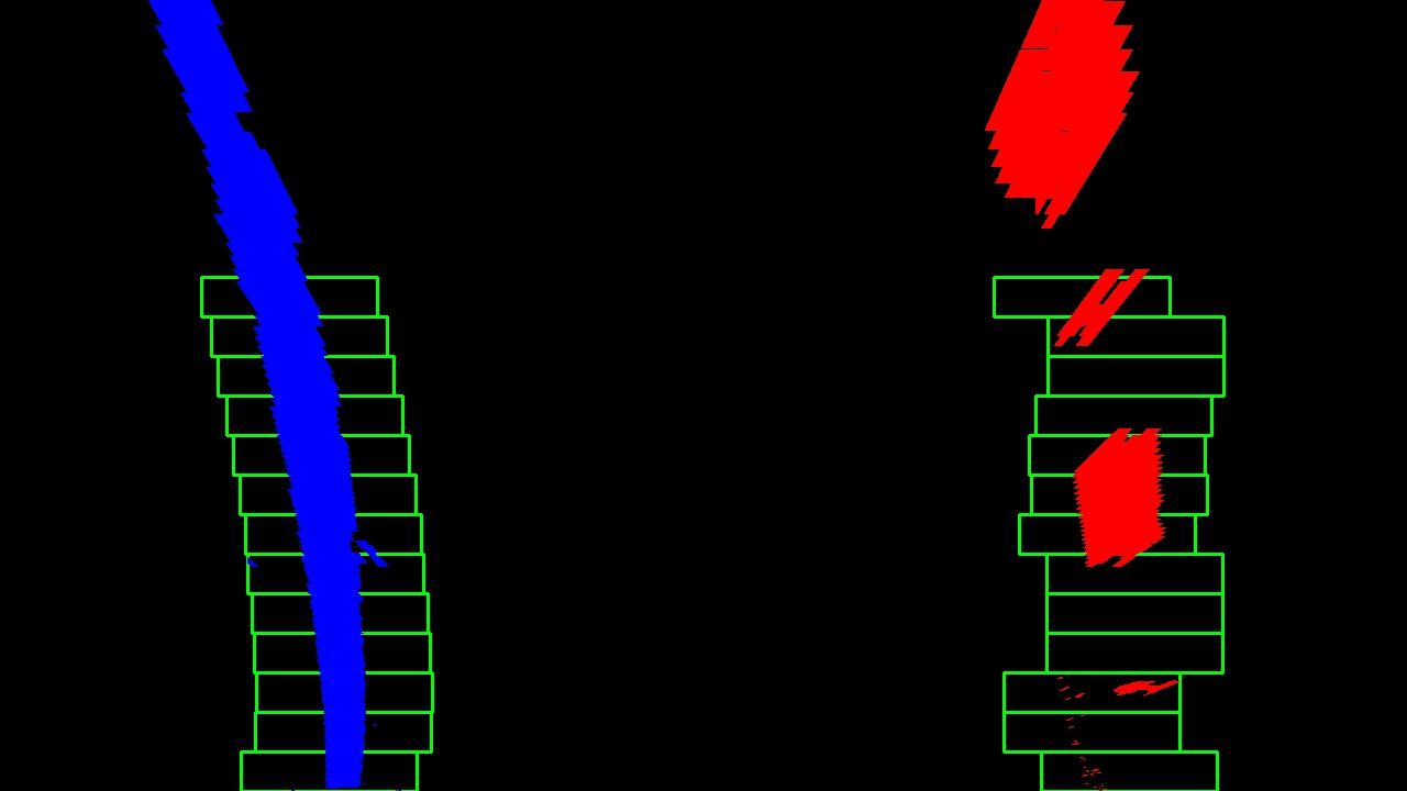
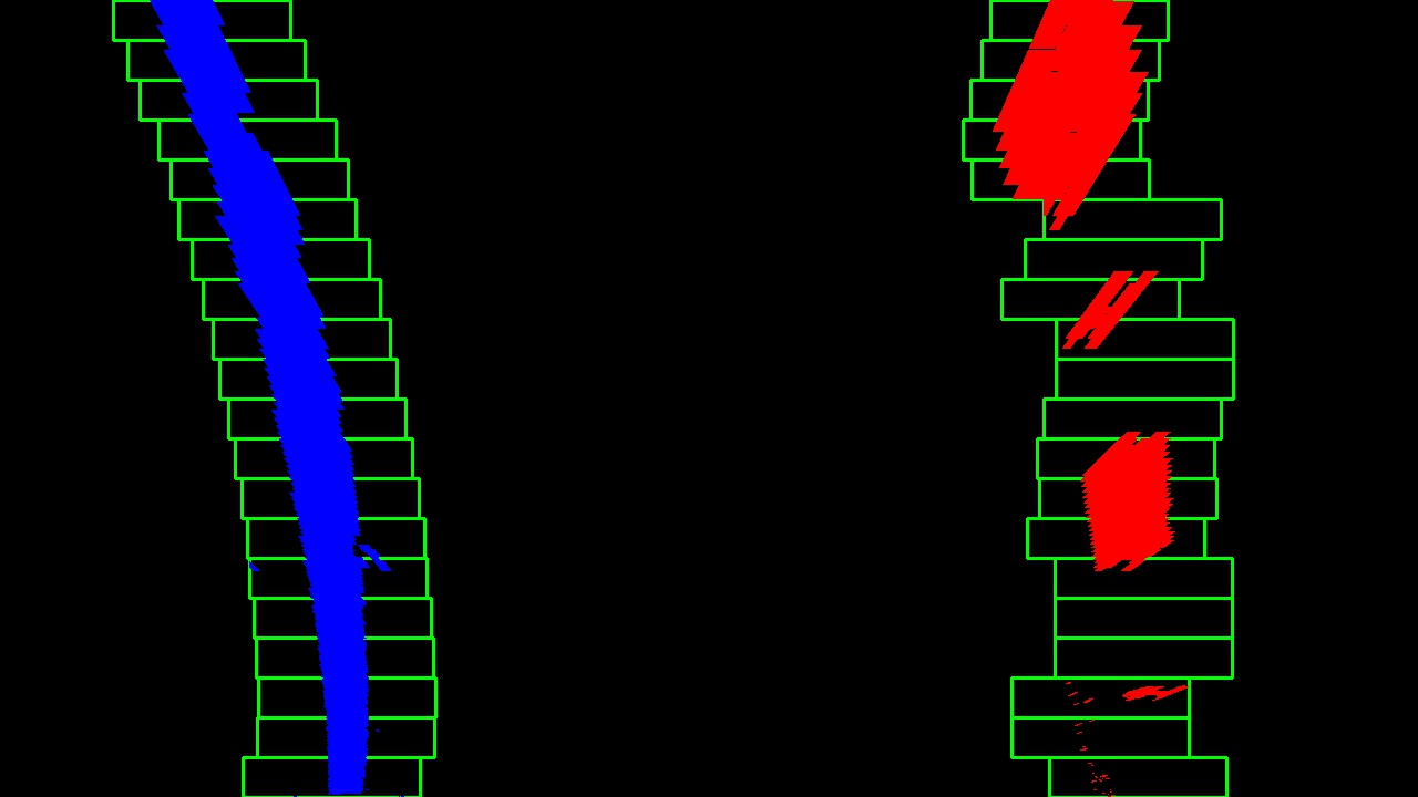
Now that we have found all our pixels belonging to each line through the sliding window method, it’s time to fit a polynomial to the line:
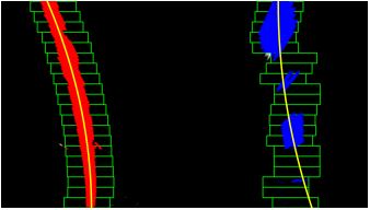
And this is the fitting line whose coefficients we need to measure the lane curvature using the formula above.
Using the full algorithm and starting fresh on every frame is inefficient, as the lines don’t move a lot from frame to frame. When performed on a video, in the following frame it’s better to search in a margin around the previous line position. This way, once we know where the lines are in one frame of video, we can do a highly targeted search for them in the next frame.


